Kalyn: a self-hosting compiler for x86-64
Over the course of my Spring 2020 semester at Harvey Mudd College, I developed a self-hosting compiler entirely from scratch. This article walks through many interesting parts of the project. It’s laid out so you can just read from beginning to end, but if you’re more interested in a particular topic, feel free to jump there. Or, take a look at the project on GitHub.
Table of contents
- What the project is and why it exists
- About the language being compiled
- Preliminary technical design decisions
- Compiler architecture walkthrough
- How I implemented it
- Worst/funniest debugging experiences
- What next?
What the project is and why it exists
Kalyn is a self-hosting compiler. This means that the compiler is itself written in the language that it knows how to compile, and so the compiler can compile itself. Self-hosting compilers are common, one reason being that programmers working on a compiler for language X probably enjoy writing code in language X and so are inclined to implement the compiler in language X.
Kalyn compiles a programming language of my own design, also called Kalyn. One obstacle to developing a self-hosting compiler for a new programming language is that in order to compile the compiler for the first time, you have to already have a compiler: it’s a chicken-and-egg problem. The simplest way to solve this problem is to first write a simple version of your compiler in a different language, and then use that compiler to compile your real compiler. So there are two implementations of the Kalyn compiler: one in Haskell and one in Kalyn itself. First I use the Haskell implementation to compile the Kalyn implementation, and then after that I can use the Kalyn implementation to compile itself.
I was inspired to create Kalyn by my Compilers class at Harvey Mudd College. In this class, students develop a working compiler for a simple Swift-like programming language over the course of the semester. However, I was left wanting more, for a few reasons:
- Most of the compiler was designed and implemented already, with only a few parts left as homework. This was probably a great idea for maximizing the ratio of learning to work, but I’m the kind of person who gets a lot of satisfaction from doing things from scratch.
- The language we compiled in class was not really fully-featured enough to do any serious work. Furthermore, the programming style of Swift and similar languages does not really “spark joy” for me, even if it’s a good idea for effective software engineering. I prefer working in more expressive languages like Haskell and Lisp when I’m not on the clock. I did not feel terribly motivated in creating a compiler for a language that I would not actually want to use.
- The compiler we worked on in class was not truly “full-stack”, as it were, since it reused a number of existing software components. For example, we used the GNU linker and assembler so that we could generate x86-64 assembly code in text format rather than binary format, and we took advantage of the C standard library to avoid having to implement memory management and input/output primitives. Again, this was probably a good idea from an educational perspective, but I wanted to take on the entire vertical from source code to assembly opcodes.
Kalyn addresses these problems in the following ways:
- I created everything from scratch, including the linker, the assembler, and the standard library. Every single byte that ends up in the executable binary is directly generated by my code.
- I designed Kalyn to make it as usable as possible while being as easy to compile as possible. It has very few core features (for example, no lists, arrays, maps, or classes), yet is truly a general-purpose programming language because these features can be implemented in user code without needing special compiler support. By aiming for a self-hosting compiler, I forced myself to prioritize language usability, because I needed to write an entire compiler in Kalyn.
- I honestly think Kalyn is a good programming language and I enjoy writing code in it. It is similar to Haskell, but uses Lisp syntax, which is something that I have seen only rarely. But since I really like Haskell except for the syntax (which I consider an absolute abomination), Kalyn adds something on top of languages that already exist, so it feels like I am creating value. (Yes, obviously Kalyn won’t be used in any real projects, but it was important to me that my language couldn’t be described as “basically the same as X, but it doesn’t work as well”.)
Kalyn by the numbers
So does it actually work? Yes! Kalyn can compile itself. The performance is slow enough to be annoying, but not slow enough to be a problem, when compared with Haskell. Here are the stats:
- Time for GHC to compile my Haskell implementation: 13 seconds
- Time for my Haskell implementation to compile my Kalyn implementation: 2 seconds
- Time for my Kalyn implementation to compile itself: 48 seconds
So we can see that Kalyn runs about 25 times slower than Haskell, which I am pretty satisfied with given that Haskell has been optimized by experts for decades and for Kalyn I basically threw together the simplest thing that could possibly work.
Now here’s a different numerical perspective, the size of the project as a function of time. The final total is 4,300 lines of Haskell code across 23 modules and 5,400 lines of Kalyn code across 43 modules. (Why more Kalyn? The syntax is slightly less concise, but mostly it’s because I had to implement the entire Haskell standard library – or at least the part I used in the compiler.) Here’s are graphs showing lines of code and number of modules over time, from which you can see I definitely left everything to the last minute…
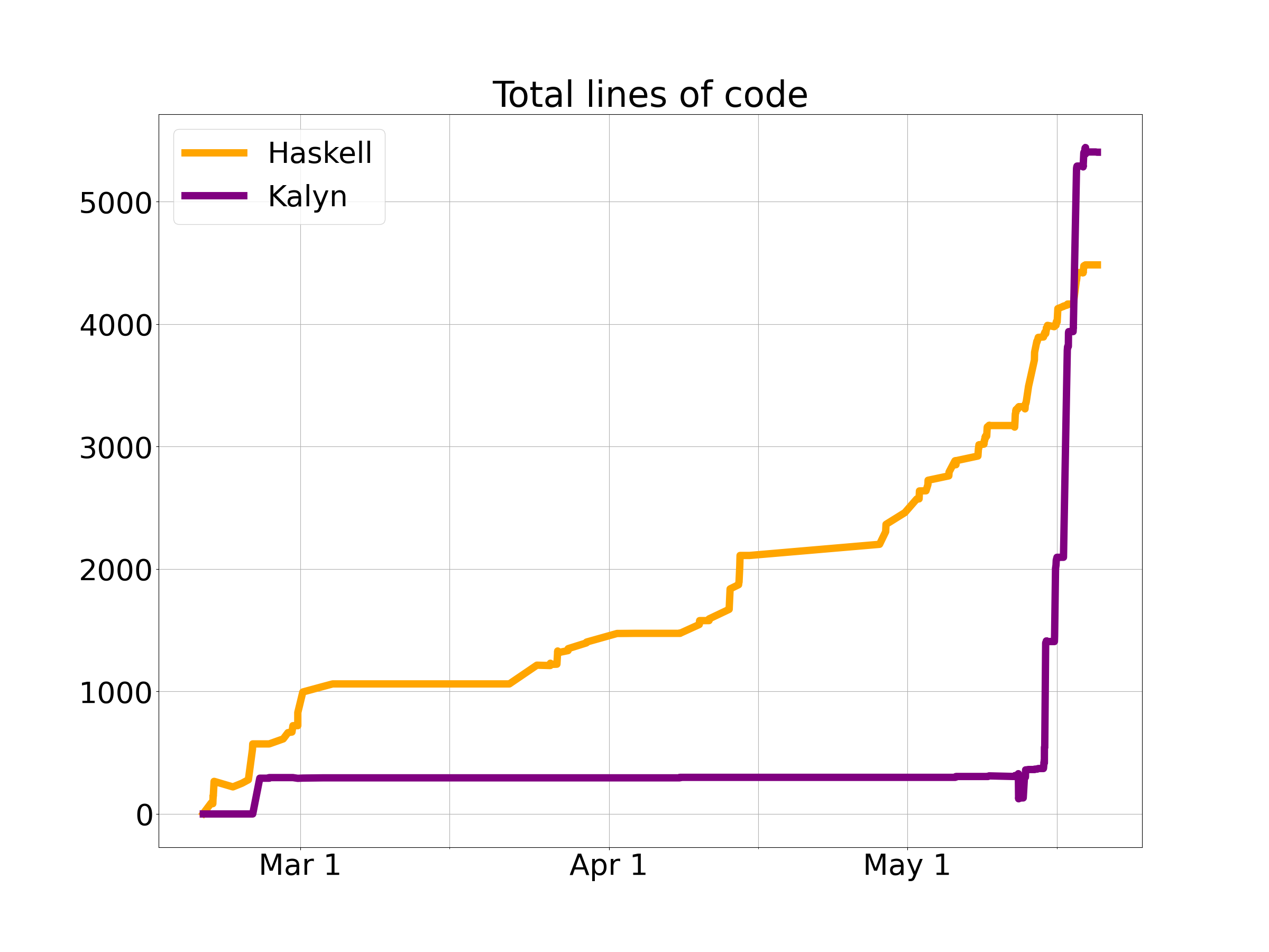
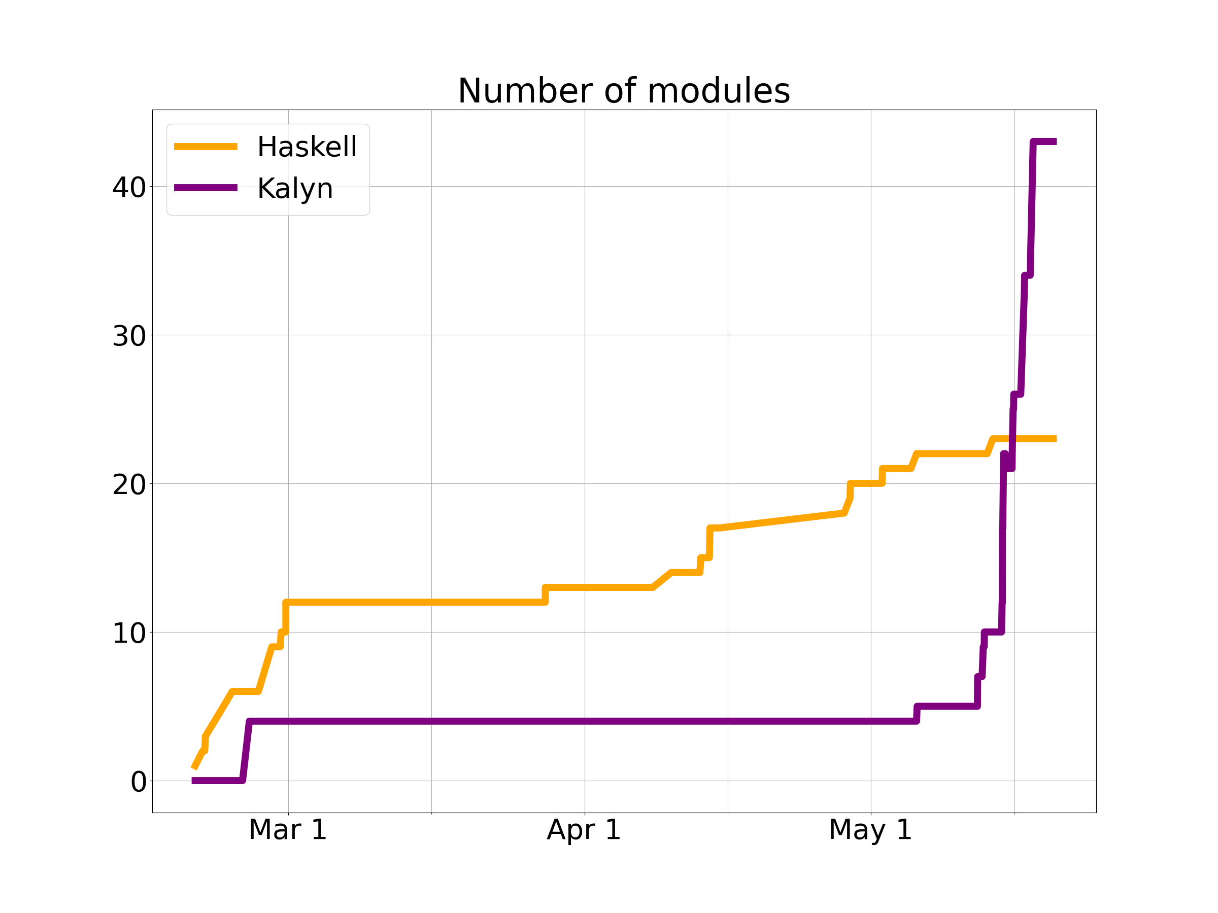
For another perspective on the development process, here is a graph of the cumulative total lines of code added and removed (so the project size at any given time is the vertical distance between the lines).
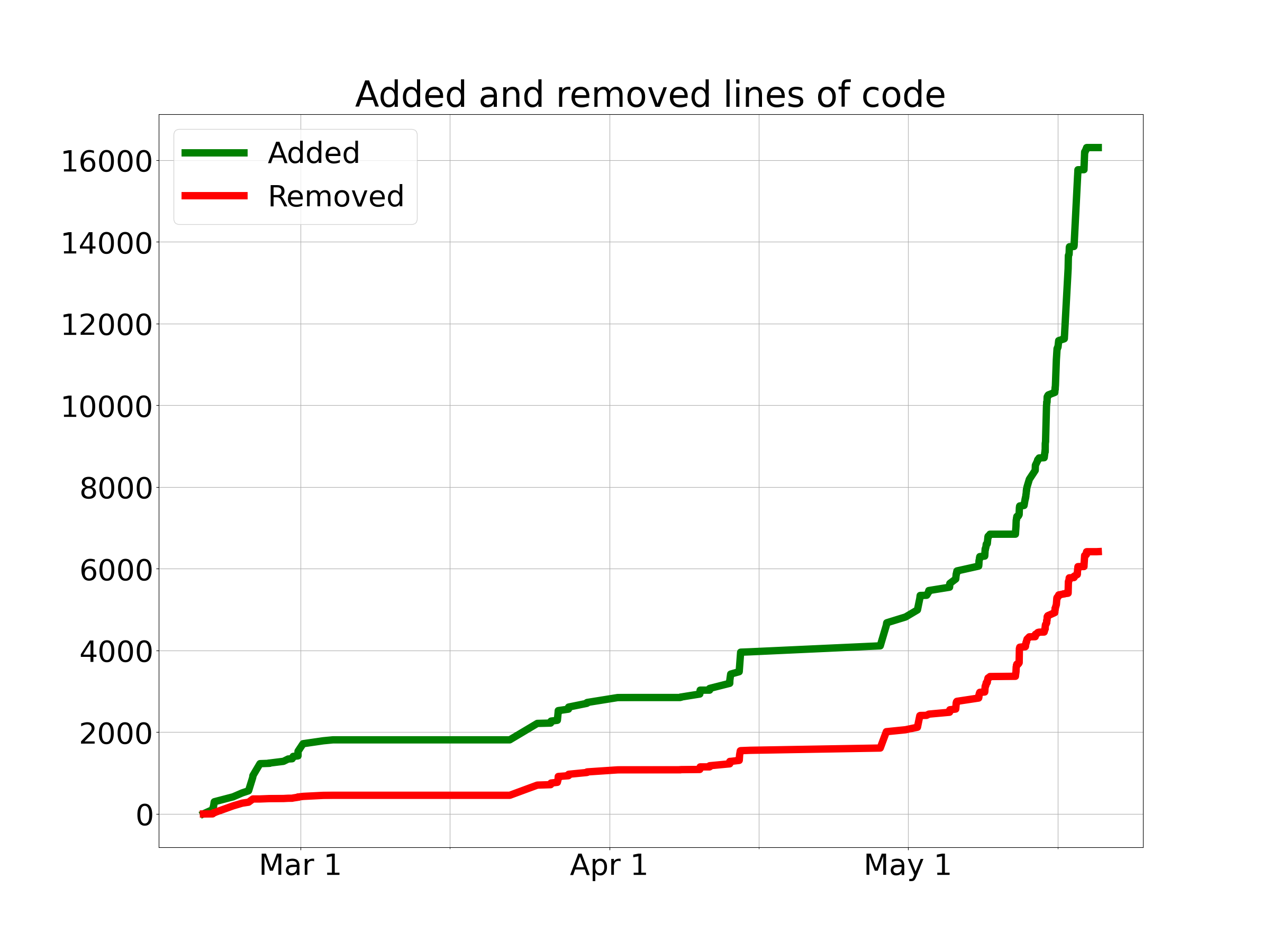
You can take a look for yourself on GitHub.
Now let’s get into the Kalyn programming language!
About the language being compiled
Kalyn is a combination of Haskell and Lisp. Here is an example of some Haskell code that prints out the prime numbers up to 100:
module Main where

-- | Check if the number is prime.
isPrime :: Int -> Bool
isPrime num =
  let factors = [2 .. num - 1]
  in  all (\factor -> num `mod` factor /= 0) factors

main :: IO ()
main =
  let nums   = [2 .. 100]
      primes = filter isPrime nums
  in  print primes
Here is the same code in Clojure, a recently developed Lisp that runs on the JVM.
(ns hello-world.core)

(defn prime?
  "Check if the number is prime."
  [n]
  (let [factors (range 2 n)]
    (every?
     (fn [factor]
       (not (zero? (mod n factor))))
     factors)))

(defn -main
  []
  (let [nums (range 2 100)
        primes (filter prime? nums)]
    (println primes)))
And here is the equivalent Kalyn code, which you can see combines the idea of Haskell with the syntax of Lisp:
(import "Stdlib.kalyn")

(defn isPrime (Func Int Bool)
  "Check if the number is prime."
  (num)
  (let ((factors (iterate (+ 1) 2 (- num 2))))
    (all
      (lambda (factor)
        (/=Int 0 (% num factor)))
      factors)))

(public def main (IO Empty)
  (let ((nums (iterate (+ 1) 2 98))
        (primes (filter isPrime nums)))
    (print (append (showList showInt primes) "\n"))))
The language is actually quite small, so we can go through all of it pretty quickly. Let’s take a look.
Data types
Kalyn is a statically typed programming language, like Haskell. It has exactly four classes of data types:
- Signed 64-bit integer, denoted
Int - Function, denoted
Func a b - Input/output monad, denoted
IO a - User-defined algebraic data types
Some more explanation is clearly in order.
Integers
Why only one size of integer? This makes the code generation easier because every integer has the same size. In fact, I designed Kalyn using what is called a boxed memory representation, so that every data type has the same size. More on this later.
What about characters? These are actually just stored as integers. This wastes a lot of space, because 56 bits out of 64 are left unused, but again it makes the implementation much simpler if we don’t have to worry about differently-sized data types.
Functions
Kalyn has first-class functions, meaning that code can dynamically create functions at runtime and pass them around just like any other data type. This is required to support any reasonable functional programming. Kalyn’s functions have closures, which requires special compiler support. More on that later.
All functions in Kalyn are automatically curried, like in Haskell. This means that all functions take only a single argument; multiple-argument functions are implemented as a single-argument function that returns another single-argument function that returns another function, and so on. I made this decision for two reasons: firstly, because currying is awesome, and secondly, because it simplifies the type system and code generation if functions all take the same number of arguments.
Because functions are curried, the notation Func a b c is really
just shorthand for Func a (Func b c), where a, b, and c are
type parameters that might stand for things like Int and List String and Func String Int.
One thing you might be wondering is how functions of no arguments are handled. The answer is there is no such thing. Since evaluating a function has no side effects (see the next section on monadic IO), there’s no difference between a function of no arguments that returns some expression and just that expression itself.
Input/output monad
Kalyn adopts Haskell’s abstraction of
monads with
youthful exuberance. Explaining monads is beyond the scope of this
article, but the point is that every input/output function in the
standard library (print, readFile, writeFile, etc.) doesn’t
actually do IO. Instead, it returns an instance of the IO monad which
represents the IO action. These instances can then be chained
together using functional programming techniques, and the result is
executed only if it is returned from the main function of the
program.
Each instance of the IO monad has a return type, as in Haskell, so the
type is denoted IO Int or IO (List String) or IO a in general.
You might think that using monadic IO is in conflict with the design goal of making Kalyn as easy as possible to compile. You would be correct. But it’s so cool!
User-defined algebraic data types
You may have noticed that most useful data types, such as booleans and lists, are absent from Kalyn. This is because you can easily define them yourself. This is done just as it is in Haskell, with algebraic data types. Here is how the Kalyn standard library defines some handy data types which will be familiar to the Haskell programmer:
(public data Bool
  False True)

(public data (Maybe a)
  Nothing (Just a))

(public data (Either l r)
  (Left l) (Right r))

(public data (Pair a b)
  (Pair a b))

(public data (List a)
  Null (Cons a (List a)))

(public alias Word8 Int)

(public data Char (Char Word8))

(public alias String (List Char))
So, for example, a variable of type List Int could be any of:
NullCons 5 NullCons 5 (Cons 2 Null)Cons 5 (Cons 2 (Cons 9 Null))- etc.
By including support for arbitrary algebraic data types, the compiler doesn’t need any special support for booleans, lists, arrays, maps, pairs, optionals, or anything else that would complicate the implementation.
Syntax
Kalyn consists of declarations and expressions, both of which are similar to Haskell except in appearance.
Expressions
First we have function calls, which are lists. Function currying is
handled automatically, so that (map (+ 1) elts) means we call the
+ function with the argument 1 and then pass that to the map
function, and take the function returned from map and pass it the
argument elts.
Next, you can define anonymous functions using lambda, so a more
explicit form of the previous code would be:
(map
  (lambda (x)
    (+ x 1))
  elts)
The type checker includes a constraint solver, so it can automatically figure out the types of anonymous functions; there’s no need to specify that manually (and, for simplicitly, you can’t).
Lambdas can have multiple arguments, but that just means they are
automatically curried, so that (lambda (x y) ...) is the same as
(lambda (x) (lambda (y) ...)).
You can establish local bindings using let:
(let ((nums (iterate (+ 1) 2 98))
      (primes (filter isPrime nums)))
  (print (showList showInt primes)))
Each binding is evaluated in sequence, and it can refer to not only previous bindings but also itself recursively. This allows you to define recursive anonymous functions:
(let ((explode
       (lambda (x)
         (explode (+ x 1)))))
  (explode 0))
Mutual recursion is
notably not supported in let bindings, because internally a let
form with multiple bindings is translated into a series of nested
single-binding let forms, which makes the code generation easier.
The last special form is case, which (as in Haskell) allows you to
return different values depending on an algebraic data type. Arbitrary
patterns of data constructors and variables can be used on the
left-hand side of each branch. For example, here is Kalyn’s
implementation of the classic unzip function from Haskell:
(public defn unzip (Func (List (Pair a b)) (Pair (List a) (List b)))
  (pairs)
  (case pairs
    (Null (Pair Null Null))
    ((Cons (Pair left right) pairs)
     (let (((Pair lefts rights)
            (unzip pairs)))
       (Pair (Cons left lefts)
             (Cons right rights))))))
You may notice that the let form employs destructuring, which is
basically the same as the pattern-matching used in case branches.
This can be done in function arguments as well, and the @ syntax
from Haskell allows you to name a value while simultaneously
destructuring it:
(lambda (c@(Char i))
  (if (isAlphaNum c)
    [c]
    (append "_u" (showInt i))))
Macros
That’s it for the core expression types in Kalyn. There are a few more
pieces of syntax, which the parser handles as macros. For example, the
if statement
(if b
  False
  True)
translates into:
(case b
  (True False)
  (False True))
The list literal [1 2 3] translates into:
(Cons 1 (Cons 2 (Cons 3 Null)))
The string "Hello" translates into:
(Cons
  (Char 72)
  (Cons
    (Char 101)
    (Cons
      (Char 108)
      (Cons
        (Char 108)
        (Cons
          (Char 111)
          Null)))))
The variadic and and or forms translate down to nested case
forms. And finally, we have the classic do notation from Haskell,
which translates into a sequence of >>= invocations. Now, as I’ll
discuss later, Kalyn doesn’t have typeclasses, which means there are
separate >>=IO, >>=State, etc. functions for each monad. As a
result, you have to specify which monad you’re working with at the
start of the macro. It looks like this:
(do IO
  (with contents (readFile "in.txt"))
  (let reversed (reverse contents))
  (writeFile "out.txt" reversed)
  (setFileMode "out.txt" 0o600))
The with form is equivalent to Haskell’s <- operator, while the
let form is the same as in Haskell. Other forms are assumed to be
monad instances whose return values are ignored (except for the last
form, which determines the return value of the entire do macro). The
above code translates like this:
(>>=IO
  (readFile "in.txt")
  (lambda (contents)
    (let ((reversed (reverse contents)))
      (>>=IO
        (writeFile "out.txt" reversed)
        (lambda (_)
          (setFileMode "out.txt" 0o600))))))
By implementing many familiar language features as macros instead of true expressions, I was able to greatly simplify the implementation of the compiler, since only the parser needs to know about these features.
You might wonder why let isn’t implemented as a macro as well, since
after all (let ((foo bar)) ...) is equivalent to ((lambda (foo) ...) bar). The answer is that this would introduce a huge amount of
overhead, because a let can be easily translated into just a single
move instruction in the assembly, whereas a function call (especially
with proper handling of closures) is much more expensive.
Declarations
First we have def, which allows you to define the value of a symbol,
giving its type and an optional
docstring, like:
(def pageSize Int
  "The page size of the CPU."
  0x1000)
Next up is defn, which is for defining functions:
(defn fst (Func (Pair a b) a)
  ((Pair a _))
  a)
Actually, though, defn is just a macro that expands to def and
lambda, like so:
(def fst (Func (Pair a b) a)
  (lambda ((Pair a _))
    a))
We have algebraic data type declarations, as we’ve seen before:
(data (Function reg)
  (Function Int Label (List (Instruction reg))))
And we have type aliases. This is the type keyword from Haskell.
(The newtype keyword is basically the same as data, and Kalyn
doesn’t care about the difference, so it doesn’t have a separate
declaration type for that.) So, for example, String can be used as a
shorthand for List Char:
(alias String (List Char))
Kalyn’s standard library defines a number of aliases, like these:
(alias Int8  Int)
(alias Int16 Int)
(alias Int32 Int)
(alias Int64 Int)

(alias Bytes String)
(alias FilePath String)
Of course, there is only one size of integer, and there is no distinction between binary and text strings, but using the type aliases is helpful to make the type signatures easier to understand.
Module system
The Kalyn compiler and standard library is split into many different files. One file is designated by the compiler as the main module, and it can import others, like:
(import "Stdlib.kalyn")
Now each declaration keyword (def, defn, data, alias) can be
optionally preceded by public to indicate that the declaration
should be made available to other code that imports the module. As an
aside, this solves a big annoyance I have with Haskell, which is that
there’s no way to specify which functions in a module should be public
without having to list all of them at the top of the file.
Ideally, Kalyn would also have a way to hide or select specific
symbols on an import, but in the interest of simplicity we don’t have
that. Qualified imports would be another useful feature, but in their
absence we get along fine by just prefixing names to avoid conflicts,
like for example mapInsert versus setInsert.
One key feature is that even the import keyword can be preceded by
public to indicate that all the imported symbols should be
re-exported. This allows for Stdlib.kalyn to public import many
submodules, so that user code only needs to import Stdlib.kalyn to
get the entire standard library.
The module system in Kalyn is really dirt simple. There’s no concept of a search path or project root. Kalyn modules are just files containing Kalyn source code (even the file extension doesn’t matter), and imports are simply resolved as filenames relative to the directory containing the module with the imports. This simplified the implementation; languages like Python impose stronger conventions on module layout but we don’t need that to get a compiler working.
Typeclasses
You may have noticed the conspicuous absence of one key feature of
Haskell, namely
typeclasses. This is
because it turns out that you don’t need them to get a compiler up and
running, even though they are really really nice. In Haskell, you can
define a Show instances like this, for example (if they weren’t
already defined in the standard library):
instance Show Bool where
  show False = "False"
  show True = "True"

instance Show a => Show (List a) where
  show elts = "[" ++ intercalate "," (map show elts) ++ "]"

show [False, True]  -- "[False,True]"
In Kalyn, we can do the same thing, we just have to define a different function for each type:
(alias (Show a) (Func a String))

(defn showBool (Show Bool)
  (bool)
  (case bool
    (False "False")
    (True "True")))

(defn showList (Func (Show a) (Show (List a)))
  (show elts)
  (concat
    ["[" (intercalate ", " (map show elts)) "]"]))

showList showBool [False, True]  ; "[False, True]"
Not ideal, but it kind of looks like the Haskell version if you
squint, and in practice it’s not that big of a pain. What’s more
annoying is that this approach doesn’t work for higher-kinded
typeclasses
like Monad. (Try it and see!) So it’s not possible to define a
function after the style of showList that would act on an arbitrary
monad if you passed it the relevant >>=Whatever bind operator.
Luckily, we only use two monads (IO and State) in the compiler, so
that wasn’t too big of a deal.
In retrospect, I’m pretty happy with the result. Extending the type checker to support typeclasses would be quite complex, so I think the limited version that I implemented was a good compromise to get a self-hosted compiler initially off the ground.
Laziness
The other major difference from Haskell that’s worth mentioning is laziness. Haskell is very lazy by default, so expressions are only evaluated when they need to be. This often wreaks havoc with evaluation order and makes it hard to understand what is running when, although it does enable some neat tricks like being able to manipulate infinite lists. Kalyn takes a simpler approach and evaluates everything eagerly. There are two main disadvantages to doing things this way:
- You can’t have infinite lists anymore, so idioms like
take 100 (iterate (+ 1) 0)don’t work. I made theiteratefunction in the standard library take an extra argument that controls the number of iterations, so we can write(iterate (+ 1) 0 100)instead and it works great. Turns out that laziness isn’t actually needed all that often, at least in this kind of project. - Normally the way lazy evaluation works is that each expression is turned into a thunk whose value can be computed when needed and then cached. By not implementing any of this, we lose the caching. That means the values of top-level symbols are actually recomputed every time they’re needed, which is unfortunate in some cases where a top-level symbol is assigned the result of a nontrivial calculation. But in the end it’s not that bad. This problem could be fixed at some additional complexity cost, even if laziness weren’t added.
… And that’s it for Kalyn! You now know the entire language.
Preliminary technical design decisions
Before we get into the compiler stack, we need to talk about a few design decisions that have a big influence on how the low-level code being generated looks.
In-memory data representations
The first choice I needed to make was how to represent each of the data types in memory, since the assembly code I generate operates directly on bytes, not monads and algebraic data types.
To simplify the implementation as much as possible, I selected a boxed memory representation. In this representation, every data type has exactly the same size, namely eight bytes (which we call a word). So, if a data type needs eight or fewer bytes, we can just store it directly like that. If it needs more, however, then instead we allocate memory for it on the heap and store a pointer to that memory. If an object has sub-objects in its fields, we can store those sub-objects in the same way: either directly, if they are small enough, or through a pointer.
Now let’s talk about the individual classes of data types. Integers are easy: since they are 64-bit, we can store them as-is in one word. The other types are more interesting.
Functions
Function objects must include two things: firstly, the address of their machine instructions in memory; secondly, the arguments in their closure. For example, suppose we run the following code:
(let ((x 5)
      (y 7))
  (lambda (z)
    (+ (* z x) y)))
Then the function object returned needs to store two values in its
closure, x = 5 and y = 7. In Kalyn, function objects consist of
three parts:
- First comes a word that contains the address of their code. (For
each
lambdaform that appears in the source code, we generate one function in the assembly, so that each lambda has a place where its instructions are stored.) - Next comes a word that specifies how many values are in the closure of the function. In theory this could be determined automatically by looking at the function address, since the size of each lambda’s closure is known at compile-time, but that would impose a lot of complexity at runtime.
- Finally, we have one word for each of the closure values. This means that function objects have different sizes, but because we put them behind a pointer, we can treat them as if they are all a single word.
Note that the order of closure arguments is important! As I explain later, the translator (code generator) arranges for the caller and the callee to agree about what order the values should go in.
In summary, the function object from above might look like this on the heap, and we would pass around a pointer to it:
  code addr   num params  value of x  value of y
  .           .           .           .
  .           .           .           .
  .           .           .           .
+-----------+-----------+-----------+-----------+
| 0x821ad   | 2         | 5         | 7         |
+-----------+-----------+-----------+-----------+
IO monad
I was a bit scared of figuring out exactly how to implement monadic IO, because it seemed very abstract. It turns out, however, to be shockingly simple. An instance of the IO monad is simply a function object which, when called, does the IO.
Let’s look at an example. Suppose we want to translate this code:
(let ((fname "test.txt")
      (msg "Hello, world!\n"))
  (writeFile fname contents))
We would end up with a function object that looks like this (where
fname and contents are pointers into the heap):
  code addr   num args    fname ptr   msg ptr
  .           .           .           .
  .           .           .           .
  .           .           .           .
+-----------+-----------+-----------+-----------+
| 0xcf73a   | 2         | 0x2eb2820 | 0x49f7988 |
+-----------+-----------+-----------+-----------+
This looks very similar to the function objects based on lambda
forms, but conceptually it’s actually rather different. Instead of
closure values, we have function arguments. With the lambda example
from before, calling the function object meant giving the code both
values from the closure together with the actual argument of the
lambda. With this example, there’s no closure and no extra argument to
provide: all the necessary information to do the IO is right there in
the function object. Despite these differences, though, the mechanics
are similar enough that both kinds of function objects can be treated
the same by Kalyn internally.
In the example above, the code address is not the address of
writeFile, because writeFile is the function that returned this
monad instance (aka function object). Instead, it’s the address of a
helper function writeFile__unmonadified which actually writes the
file. Each function that returns a monad has an associated helper
function to do the work.
Now let’s consider how we implement the monadic binding operator
>>=IO. The >>=IO function itself is just a wrapper that returns a
function object pointing at >>=IO__unmonadified which does the
actual work. What is that actual work? The helper gets two arguments
ma and famb. First, it runs ma to do its IO and procure the
return value. Then it passes that return value to famb to get
another function object which is the returned IO instance. Finally, it
must invoke that function object to do the rest of the IO (which
might constitute further invocations of >>=IO) before returning.
Finally, since something must kick off the IO execution in the first
place, the boilerplate code generated for Kalyn’s main function
first evaluates its body to get a monad instance and then invokes that
function object to do all the IO. Then it exits to terminate the
process.
User-defined algebraic data types
This is perhaps best illustrated by example. First consider booleans:
(data Bool
  False True)
The value False is represented as 0 and the value True is
represented as 1. There’s no extra data, so we don’t need a pointer.
Now let’s look at optionals:
(data (Maybe a)
  Nothing (Just a))
We can’t fit this into a single word without getting creative, and
creative is not compatible with simple, so we use a pointer for this
one. The first word on the heap is an integer that tells us which
constructor is being used, just like with booleans (0 for Nothing, 1
for Just). For Nothing, that’s it. For Just, however, the 1 is
followed by another word that contains the a in the Just a. This
could be either a piece of literal data or a pointer to more
heap-allocated data. This might seem like a waste of space in the case
of Nothing, but (without being creative) we need to have exactly one
place to look to find out whether we have a Nothing or a Just, so
either every constructor has to fit in a word or we have to put all of
them behind a pointer.
At this point you’ve seen almost everything. In general, an algebraic data type consists of two parts:
- A header word to tell you which constructor was used. This is
omitted if there’s only one constructor, such as in
Char. - If the constructor has fields, then the values of the fields.
If the combination of those two parts fits inside one word for every data constructor, then the type can be stored directly without a pointer. Otherwise, we use a pointer for every constructor. In case you’re curious, we need a pointer when either:
- any of the constructors has more than one field
- any of the constructors has at least one field, and there’s more than one constructor
(What about (data Empty), with no constructors at all? Eh… we just
use a zero. We could be smart and elide empty fields from containing
data constructors, but this would complicate the implementation.)
Calling convention
Okay, so now we know how Kalyn’s data types are represented. One notable omission, however, is how to actually use function objects.
One of the first decisions I needed to make after deciding on data types was to establish the Kalyn calling convention. This describes the way in which functions receive their arguments from callers, and how they return results.
In Kalyn, function arguments are passed on the stack. Here is the layout of a single stack frame:
| Previous stack frame |
+----------------------+
| Function argument 1  |
| Function argument 2  |
|         ...          |
+----------------------+
|    Return address    |
+----------------------+
|  Saved base pointer  | <-- base pointer
+----------------------+
|   Local variable 1   |
|   Local variable 2   |
|         ...          |
+----------------------+
|   Saved register 1   |
|   Saved register 2   |
|         ...          | <-- stack pointer
+----------------------+
|   Next stack frame   |
As is standard in x86 assembly, two registers are used to manage the
stack: the stack pointer (%rsp) and the base pointer (%rbp). The
stack pointer always points to the last item that was pushed onto the
stack (which will be at the bottom of the stack, since in x86 the
stack grows downward). The base pointer, on the other hand, points to
a fixed point within the stack frame and does not change as items are
pushed and popped (at least until a new stack frame is entered). The
base pointer is used to easily locate specific values within the stack
frame, since indexing from the stack pointer would be difficult (as it
moves around within the frame).
Here is the flow of a function call:
- The caller pushes all of the arguments for the function onto the stack. For regular function objects, this means all the closure values followed by the main parameter of the function. For IO functions, this just means the actual arguments of the function.
- The caller invokes the function using the
callqx86 instruction. This automatically pushes a return address onto the stack and jumps into the function. - The callee pushes the current base pointer (which pointed into the caller’s stack frame) onto the stack, in order to save its value, and then updates the base pointer to point at the current stack pointer. Now the base pointer can be used to index into the callee’s stack frame.
- If the callee can’t fit all of its variables into registers (as I discuss later in the section on register allocation), it moves the stack pointer further downward to reserve stack space for the extra variables.
- The callee pushes the values of any registers it uses onto the stack, in order to save their values.
- The callee’s function body is executed. When it needs access to the function arguments or local variable space, it can locate them using the base pointer. If the callee needs to call more functions (quite likely), it pushes their arguments and this process repeats recursively.
- The callee pops the values of the saved registers off the stack, restoring their values for the caller.
- The callee moves the stack pointer upwards to deallocate the space it reserved for its local variables.
- The callee pops the saved base pointer off the stack. The base pointer now points back into the caller’s stack frame.
- The caller puts its return value into the
%raxregisters, then returns using theretqx86 instruction. This pops the return address off the stack and jumps back to the caller. - The caller moves the stack pointer up to deallocate the space it used to push the function arguments.
In the stack frame diagram above, the base pointer and stack pointer will be at the places labeled while the callee’s function body is executing.
Notice that the callee’s base pointer is pointing at the saved base pointer from the caller. That base pointer points at the saved base pointer from the caller’s caller, and so on. Thus, by traversing the chain of base pointers, we can construct a call stack. All we need to do is look right above each base pointer to find the return addresses, and that will tell us which functions we are in (and at which instruction, which can be translated into a line number). Of course, Kalyn does not actually provide backtraces at runtime, but the ability to follow the base pointer chain was invaluable when debugging in GDB.
Aside from stack frame layout, there is one other important consideration when choosing a calling convention, which is to designate machine registers as either caller-saved or callee-saved. Since every function must do its work using the same set of registers, conflicts between different functions must be avoided. This is typically done by pushing the value of a register onto the stack, and then later popping it off to restore its value. Between the push and the pop, the register can safely be used by another function. The question is whether the caller or callee is responsible for saving the values of possibly conflicting registers.
In the standard x86-64 calling convention, some registers are marked as caller-saved and others are marked as callee-saved:
- Caller-saved:
%rax,%rcx,%rdx,%rsi,%rdi,%r8,%r9,%r10,%r11 - Callee-saved:
%rbx,%r12,%r13,%r14,%r15
This split was chosen as a compromise, because caller-saved registers
are better to use in some cases while callee-saved registers are
better for others. In Kalyn, however, all registers are callee-saved
except for %rax (which is used to store return values). This
simplifies the implementation.
Why all callee-saved instead of all caller-saved? I judged that it was simpler to arrange for registers to be saved and restored at the beginning and end of each function rather than before and after each subroutine call. But the choice is mostly one of taste.
Readers familiar with x86-64 might recall that in the standard calling
convention, arguments are not passed on the stack unless there are
many of them. The first six arguments are passed in registers, namely
%rdi, %rsi, %rdx, %rcx, %r8, and %r9. This is clearly more
efficient than pushing every argument onto the stack, because memory
accesses are slow. But, it’s more complicated, so Kalyn does things
the simple way.
Readers familiar with assembly programming might also object “doesn’t choosing a nonstandard calling convention prevent Kalyn from interoperating with other code?” Well… yes! But the goal for this project was to write everything from scratch, so in fact there is no other code to interoperate with. The only exception is system calls, which occur only within primitive functions that I hand-wrote in assembly. The rest of Kalyn doesn’t need to know about system calls, so there’s no need for it to use their calling convention.
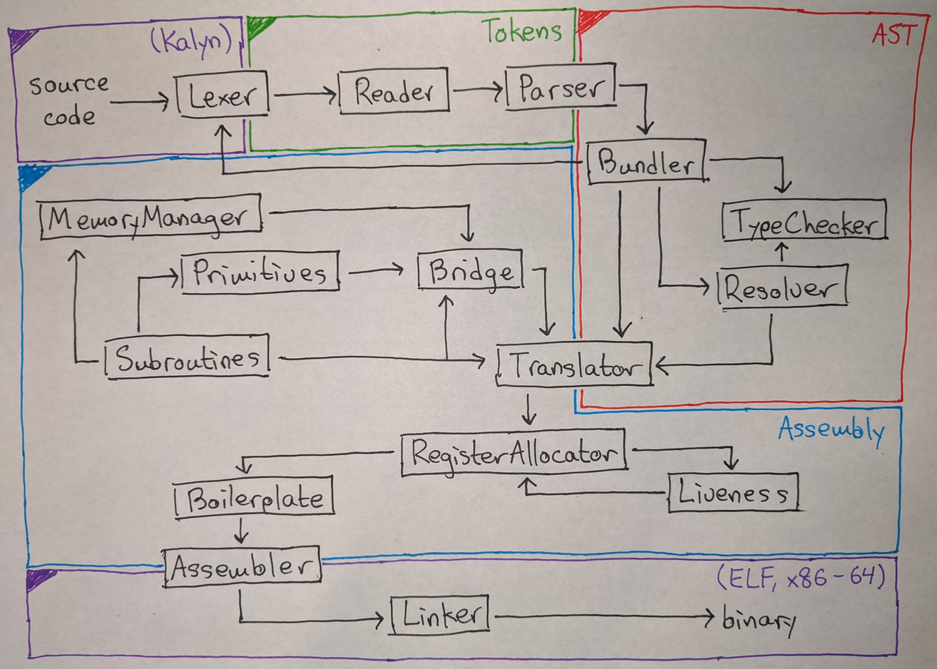
Compiler architecture walkthrough
In this section I will walk you through the entire compiler pipeline from top to bottom. Let’s follow the sample program that I used to illustrate Kalyn’s syntax:
(import "Stdlib.kalyn")

(defn isPrime (Func Int Bool)
  "Check if the number is prime."
  (num)
  (let ((factors (iterate (+ 1) 2 (- num 2))))
    (all
      (lambda (factor)
        (/=Int 0 (% num factor)))
      factors)))

(public def main (IO Empty)
  (let ((nums (iterate (+ 1) 2 98))
        (primes (filter isPrime nums)))
    (print (append (showList showInt primes) "\n"))))
The first step of the compiler is the lexer. This takes the program source code and turns it into a sequence of tokens, which are names, numbers, and pieces of punctuation. It looks like this:
LPAREN
SYMBOL "import"
STRING "Stdlib.kalyn"
RPAREN
LPAREN
SYMBOL "defn"
SYMBOL "isPrime"
LPAREN
SYMBOL "Func"
SYMBOL "Int"
SYMBOL "Bool"
RPAREN
STRING "Check if the number is prime."
LPAREN
SYMBOL "num"
RPAREN
LPAREN
SYMBOL "let"
LPAREN
LPAREN
SYMBOL "factors"
LPAREN
SYMBOL "iterate"
LPAREN
SYMBOL "+"
...
Next up is the reader. This converts the token stream into a hierarchical list-of-lists representation. In other words, it parses the Lisp syntax of Kalyn. Here is what that looks like:
RoundList
    [ Symbol "import"
    , StrAtom "Stdlib.kalyn"
    ]
RoundList
    [ Symbol "defn"
    , Symbol "isPrime"
    , RoundList
        [ Symbol "Func"
        , Symbol "Int"
        , Symbol "Bool"
        ]
    , StrAtom "Check if the number is prime."
    , RoundList [ Symbol "num" ]
    , RoundList
        [ Symbol "let"
        , RoundList
            [ RoundList
                [ Symbol "factors"
                , RoundList
                    [ Symbol "iterate"
                    , RoundList
                        [ Symbol "+"
                        , IntAtom 1
                        ]
                    ...
After the reader comes the parser, which converts the list-of-lists
representation into an abstract syntax tree
(AST) that can
be easily processed by the rest of the compiler. The AST is composed
of the declarations and expressions that I outlined earlier. Notably
it does not include any macros such as if or do, since the parser
automatically translates these into their lower-level counterparts.
Here is part of the AST for the program above:
Import False "Stdlib.kalyn"
Def False "isPrime"
    ( Type [] "Func"
        [ Type [] "Int" []
        , Type [] "Bool" []
        ]
    )
    ( Lambda "num"
        ( Let "factors"
            ( Call
                ( Call
                    ( Call ( Variable "iterate" )
                        ( Call ( Variable "+" ) ( Const 1 ) )
                    ) ( Const 2 )
                )
                ( Call
                    ( Call ( Variable "-" ) ( Variable "num" ) ) ( Const 2 )
                )
            )
            ( Call
                ( Call ( Variable "all" )
                    ( Lambda "factor"
                        ( Call
                            ( Call ( Variable "/=Int" ) ( Const 0 ) )
                            ( Call
                                ...
The False that appears after Import and Def mean that public
was not used on those declarations. The empty lists after each Type
are because this code does not use typeclass constraints. (I wrote the
parser before deciding I could get away without typeclass support for
the first version of Kalyn, so all of the AST manipulation functions
take typeclasses into account.)
One interesting thing you might note is that the parser handles
function currying, so every Call has exactly two arguments even
though functions were called with more than two arguments in the input
program.
Next up is the bundler. The lexer, reader, and parser are actually all
run from the bundler, which is the real entry point to the compiler.
The bundler is responsible for handling the module system of Kalyn.
After lexing, reading, and parsing the main module, the bundler checks
for Import forms. If it finds any, it lexes, reads, and parses the
files referenced, and continues recursively until it has processed all
of the needed source code.
At this point, the bundler resolves transitive imports. In other
words, it inspects the collection of import and public import
forms in all loaded modules and determines what modules each other
module can “see”. So, if A.kalyn has (import "B.kalyn") and
B.kalyn has (import "C.kalyn") and (public import "D.kalyn"),
then A.kalyn can see itself, B.kalyn, and D.kalyn, but not
C.kalyn.
After the bundler has finished running, it has produced a collection of modules (each with a list of declarations and information about what other modules are visible). This collection is called a bundle, surprisingly enough. Before the bundle can be transformed into assembly by the translator, it must be passed to two other side modules: the resolver and the type checker.
The job of the resolver is twofold. First it must decide on a unique
name for every object that the assembly code will need to refer to
(such as variables, functions, and data constructors). This process,
called name mangling,
entails substituting Unicode characters with ASCII equivalents and
also making sure variables by the same name in different modules don’t
conflict with each other. For example, the foldr function defined in
Stdlib/Lists.kalyn might be given the name
__src_u45kalynStdlibLists_u46kalyn__foldr.
After the resolver decides on names, it also must generate a mapping
for each module that translates names from user code into the internal
names. So, in every module that imports Stdlib/Lists.kalyn there
will be a mapping from foldr to
__src_u45kalynStdlibLists_u46kalyn__foldr. The mapping also includes
type information and, for data constructor, notes on which data
constructor is in use, how many fields it has, etc. The mappings
generated by the resolver are used to look up symbol definitions in
both the type checker and translator.
At this point the bundle is run through the type checker. It might surprise you to hear that the type checker doesn’t actually produce information for any other parts of the compiler. Its only purpose is to crash the compiler if there is a type error. You might expect that in a strongly typed programming language we would need type information in order to compile. In fact, however, my use of a boxed memory representation means that code that operates on a value doesn’t actually need to know what type that value has. This means that the only utility in the type checker is making it so that type errors will give you a compile-time error instead of a segmentation fault at runtime. (Still pretty useful though.) I took advantage of this property by not bothering to port the type checker to Kalyn. Since I already know from the Haskell implementation that my Kalyn code type-checks, and since compilation doesn’t require type information, the Kalyn implementation doesn’t need a type checker to be self-hosting. (Although obviously it will need one eventually, in order to be useful.)
Now we arrive at the core of the compiler, the translator (also called
the code generator). At this point we have a bundle that contains AST
declarations and expressions, together with a resolver mapping that
tells us the meaning of every name that appears in the AST. The job of
the translator is to transform each declaration from the AST into a
set of one or more functions in x86 assembly. Here’s part of the
translated code for isPrime from our example:
__Main_u46kalyn__isPrime:
        pushq $16
        callq memoryAlloc
        addq $8, %rsp
        movq %rax, %t0
        leaq __Main_u46kalyn__isPrime__uncurried(%rip), %t1
        movq %t1, (%t0)
        movq $0, 8(%t0)
        movq %t0, %rax
        retq
__Main_u46kalyn__isPrime__uncurried:
        movq 16(%rbp), %t2
        movq $1, %t8
        pushq %t8
        callq plus__curried0
        addq $8, %rsp
        movq %rax, %t9
        movq %t9, %t5
        pushq %t5
        movq $2, %t6
        pushq %t6
        movq %t2, %t10
        pushq %t10
        movq $2, %t11
        pushq %t11
        callq minus__uncurried
        ...
(Why two different functions? The first one returns the value of
isPrime, which is a function object, and the second one implements
the lambda for that function object.)
What ends up in the binary is, however, not only this code for user functions, but also code for the core primitives of the language. These are things like arithmetic and IO operations which can’t be implemented directly in Kalyn. We have to start somewhere! I wrote those functions manually in assembly, and they are added to the program by the translator.
There are a few modules that are responsible for dealing with primitives:
- Subroutines includes code that is used to implement common logic, like getting arguments from the stack or performing a function call.
- Primitives has implementations of all the basic primitive
functions that user code can call, like
+andprintand>>=IO. - MemoryManager has internal functions that are used to handle memory allocation. Remember, “from scratch” means no malloc!
- Bridge inspects the user code to see what primitives it calls, and links in only those primitives to avoid bloating the binary. It also handles wrapping primitives so that they are suitable to be called from user code. This includes generating curried and monadic wrappers so that I didn’t have to worry about any of that when implementing the actual primitives.
You might notice in the assembly snippet above that we are using
virtual registers %t0, %t1, etc. instead of just the typical x86
machine registers %rax, %rdi, %rsi, etc. This is because code
generation is much easier when we can pretend we have infinitely many
registers. It is the job of the register allocator to map these
virtual registers onto actual machine registers, and to move extra
information into local variables on the stack when there are not
enough machine registers to fit all the data.
The first step of register allocation is to perform a liveness
analysis. We analyze each assembly instruction to determine which
registers it reads from and writes to. Based on that information, we
can perform an iterative analysis to determine which registers are
live (might be used in the future) at each point in the program. If
two virtual registers are live at the same time, then they can’t be
assigned to the same physical register or they would conflict. Here is
part of the liveness analysis for isPrime:
__Main_u46kalyn__isPrime:

;; live IN: (none)
;; used: (none)
        pushq $16
;; defined: (none)
;; live OUT: (none)

;; live IN: (none)
;; used: (none)
        callq memoryAlloc
;; defined: %rax
;; live OUT: %rax

;; live IN: %rax
;; used: (none)
        addq $8, %rsp
;; defined: %rsp
;; live OUT: %rax

;; live IN: %rax
;; used: %rax
        movq %rax, %t0
;; defined: %t0
;; live OUT: %t0

;; live IN: %t0
;; used: %rip
        leaq __Main_u46kalyn__isPrime__uncurried(%rip), %t1
;; defined: %t1
;; live OUT: %t0, %t1

;; live IN: %t0, %t1
;; used: %t0, %t1
        movq %t1, (%t0)
;; defined: (none)
;; live OUT: %t0

...
Based on this information, the register allocator rewrites the code to
use appropriate physical registers. You can see that %t0 was placed
in %rdx and %t1 was placed in %rcx:
__Main_u46kalyn__isPrime:
        pushq $16
        callq memoryAlloc
        addq $8, %rsp
        movq %rax, %rdx
        leaq __Main_u46kalyn__isPrime__uncurried(%rip), %rcx
        movq %rcx, (%rdx)
        movq $0, 8(%rdx)
        movq %rdx, %rax
        retq
__Main_u46kalyn__isPrime__uncurried:
        movq 16(%rbp), %rsi
        movq $1, %rax
        pushq %rax
        callq plus__curried0
        addq $8, %rsp
        movq %rax, %rdx
        movq %rdx, %rcx
        pushq %rcx
        movq $2, %rcx
        pushq %rcx
        movq %rsi, %rcx
        pushq %rcx
        movq $2, %rcx
        pushq %rcx
        callq minus__uncurried
After code generation, there is one final transformation step on the
assembly, which is handled by the boilerplate module. This module
adapts each function to respect the Kalyn calling convention by
updating the base pointer, saving and restoring the data registers it
overwrites, and, if the function needed local variables, moving the
stack pointer to allocate and deallocate space for them. Here is part
of the final version of isPrime:
__Main_u46kalyn__isPrime:
        pushq %rbp
        movq %rsp, %rbp
        pushq %rdx
        pushq %rcx
        pushq $16
        callq memoryAlloc
        addq $8, %rsp
        movq %rax, %rdx
        leaq __Main_u46kalyn__isPrime__uncurried(%rip), %rcx
        movq %rcx, (%rdx)
        movq $0, 8(%rdx)
        movq %rdx, %rax
        popq %rcx
        popq %rdx
        popq %rbp
        retq
__Main_u46kalyn__isPrime__uncurried:
        pushq %rbp
        movq %rsp, %rbp
        pushq %rsi
        pushq %rdx
        pushq %rcx
        pushq %rbx
        movq 16(%rbp), %rsi
At this point we have the entire program in x86 assembly format. It is
now time for the assembler to translate each assembly instruction into
the appropriate sequence of bytes. Mechanically this is a
straightforward process, although deciphering the reference
materials is quite the task.
For example, here is the binary for each instruction in
__Main_u46kalyn__isPrime:
48 ff f5                pushq %rbp
48 8b ec                movq %rsp, %rbp
48 ff f2                pushq %rdx
48 ff f1                pushq %rcx
68 10 00 00 00          pushq $16
e8 f1 4e 01 00          callq memoryAlloc
48 81 c4 08 00 00 00    addq $8, %rsp
48 8b d0                movq %rax, %rdx
48 8d 0d 21 00 00 00    leaq __Main_u46kalyn__isPrime__uncurried(%rip), %rcx
48 89 8c 22 00 00 00    movq %rcx, (%rdx)
00
48 c7 84 22 08 00 00    movq $0, 8(%rdx)
00 00 00 00 00
48 8b c2                movq %rdx, %rax
48 8f c1                popq %rcx
48 8f c2                popq %rdx
48 8f c5                popq %rbp
c3                      retq
It’s at this point that all the labels generated by the resolver are put to use: each one is translated to a numerical offset in bytes that can be embedded into the binary.
The final step is the linker. This takes the binary code and data that was generated by the assembler and wraps it in a header in the Executable and Linkable Format (ELF). The resulting binary has metadata that is used by the operating system to load it into memory and that is used by GDB to display debugging information:
ELF Header:
  Magic:   7f 45 4c 46 02 01 01 00 00 00 00 00 00 00 00 00
  Class:                             ELF64
  Data:                              2's complement, little endian
  Version:                           1 (current)
  OS/ABI:                            UNIX - System V
  ABI Version:                       0
  Type:                              EXEC (Executable file)
  Machine:                           Advanced Micro Devices X86-64
  Version:                           0x1
  Entry point address:               0x18000
  Start of program headers:          64 (bytes into file)
  Start of section headers:          176 (bytes into file)
  Flags:                             0x0
  Size of this header:               64 (bytes)
  Size of program headers:           56 (bytes)
  Number of program headers:         2
  Size of section headers:           64 (bytes)
  Number of section headers:         6
  Section header string table index: 1

Section Headers:
  [Nr] Name              Type             Address           Offset
       Size              EntSize          Flags  Link  Info  Align
  [ 0]                   NULL             0000000000000000  00000000
       0000000000000000  0000000000000000           0     0     0
  [ 1] .shstrtab         STRTAB           0000000000000000  00000230
       0000000000000027  0000000000000000           0     0     0
  [ 2] .symtab           SYMTAB           0000000000000000  00000257
       0000000000003348  0000000000000018           3   547     0
  [ 3] .strtab           STRTAB           0000000000000000  0000359f
       00000000000045b0  0000000000000000           0     0     0
  [ 4] .text             PROGBITS         0000000000018000  00008000
       0000000000015245  0000000000000000  AX       0     0     0
  [ 5] .data             PROGBITS         000000000002e000  0001e000
       00000000000010b7  0000000000000000  WA       0     0     0

Program Headers:
  Type           Offset             VirtAddr           PhysAddr
                 FileSiz            MemSiz              Flags  Align
  LOAD           0x0000000000008000 0x0000000000018000 0x0000000000000000
                 0x0000000000015245 0x0000000000015245  R E    0x0
  LOAD           0x000000000001e000 0x000000000002e000 0x0000000000000000
                 0x00000000000010b7 0x00000000000010b7  RW     0x0

Symbol table '.symtab' contains 547 entries:
   Num:    Value          Size Type    Bind   Vis      Ndx Name
     0: 0000000000000000     0 NOTYPE  LOCAL  DEFAULT  UND
     1: 0000000000018326     0 FUNC    LOCAL  DEFAULT    4 __Booleans_u46kalyn__not
     2: 000000000001836e     0 FUNC    LOCAL  DEFAULT    4 __Booleans_u46kalyn__not_
     3: 00000000000183d5     0 FUNC    LOCAL  DEFAULT    4 __Booleans_u46kalyn__xor
     4: 000000000001841d     0 FUNC    LOCAL  DEFAULT    4 __Booleans_u46kalyn__xor_
     5: 000000000001847b     0 FUNC    LOCAL  DEFAULT    4 __Booleans_u46kalyn__xor_
     6: 000000000001f6c1     0 FUNC    LOCAL  DEFAULT    4 __DataTypes_u46kalyn__Cha
     ...
And now you know how program source code flows through the entire Kalyn compiler stack to become an executable native binary.
How I implemented it
This section has a deep dive into each part of the compiler implementation, touching on all of the interesting technical decisions that I made.
Lexer, reader, and parser
The first step in the compiler is transforming source code into an AST. I decided to split this process into three pieces, rather than the usual two (lexing and parsing) or one (doing everything in the parser). The reason is that it’s pretty easy to cleanly separate each of the three steps, and doing this makes the implementation easier to manage.
The reader, which handles the Lisp syntax of Kalyn, is implemented as a recursive descent parser. This is a pretty simple task because there is not too much syntax and the grammar is LL(1) for practical purposes. The Lisp syntax is the only part of Kalyn that requires a real recursive descent parser, and by separating it out into a separate reader module, I was able to make the parser itself trivial: it simply needs to pattern-match on the lists that it receives to decide which AST nodes they correspond to. Note that we only get the easy LL(1) grammar because the lexer runs first and converts runs of characters into single tokens. Without the lexer, reader, and parser all being separate, the implementation would be significantly more complex.
One thing to note about the lexer is that it doesn’t use regular expressions, unlike most lexers, and no part of the stack uses a lexer or parser generator. The reason for this is simple: if I had, then I would have needed to implement the dependency (regular expressions, lexer/parser generator) in Kalyn!
Standard library
- Kalyn implementation: Stdlib
By design, Kalyn omits most useful features from the core language, deferring them instead to user-defined functions and algebraic data types. So I needed to implement all of the data structures that I wanted to use in the compiler. For the most part, this was just lists, booleans, maps, and sets.
Lists and booleans were fairly easy. The main challenge was simply
implementing the large volume of standard library functions that I
needed in order to manipulate them properly. There are a total of 139
public functions in the Kalyn standard library, with almost all of the
names lifted directly from Haskell. I wrote most of them myself
because the Haskell standard library is pretty easy to implement for
the most part; for example, here is a typical function from
Stdlib/Lists.kalyn:
(public defn drop (Func Int (List a) (List a))
  (n elts)
  (if (<=Int n 0)
    elts
    (case elts
      (Null Null)
      ((Cons fst rst)
       (drop (- n 1) rst)))))
I did certainly have some tricky bugs caused by misimplemented standard library functions, though.
The main challenge – and in fact the very first thing I implemented in Kalyn, to make sure everything was working – was maps and sets. I elected to use splay trees, because they are one of the simplest self-balancing trees to implement. A data structure that did not have $$ O(n \log n) $$ operations would not be acceptable, because the Kalyn compiler makes heavy use of very large maps, and I anticipated (correctly) that Kalyn would run slowly enough to make compiler performance an issue.
In retrospect, splay trees are not actually the right choice for any standard library implementation in a functional language, because the amortized analysis of splay trees requires that lookups be able to mutate the tree. Unfortunately, this can’t be implemented in a language that doesn’t support mutation without changing the interface of map lookups, an unacceptable burden. Haskell uses size-balanced binary trees. Having noticed this problem only late into the project, I elected to hope that my trees wouldn’t perform too poorly if rebalancing on lookup were omitted. It seems to be good enough.
Self-balancing trees are quite tricky to implement, especially in a functional language, so I stole a Haskell implementation from the TreeStructures package on Hackage. It did turn out that this implementation had several bugs, which were a joy to discover while tracking down seemingly unrelated issues in the compiler, but I was able to fix them and Kalyn’s maps seem pretty robust now.
What about sets? They are just maps whose values are the Empty
algebraic data type that has one constructor and no fields. This
wastes space (each key-value mapping stores an extra zero), but that’s
hardly the worst memory offense of Kalyn, so I judged it to be fine.
The Stdlib/Collections/Sets.kalyn module has adapter functions that
wrap the map module to remove references to map values.
There’s one other interesting part of the standard library, which are
the typeclass instances. As I mentioned earlier, Kalyn doesn’t support
typeclasses at the moment, which was a bit tricky to deal with since
the Haskell implementation makes heavy use of the typeclass functions
show, compare, (==), and >>=. My approach was to make every
function with a typeclass constraint instead take an additional
parameter which is a concrete instance of the typeclass function. So,
for example, when constructing a map of strings, you pass in the
compareString function. If you want to convert a list to a string,
you call the showList function and pass it also the appropriate
showInt or showString or whatever is appropriate for your element
type. Finding the index of an integer in a list requires passing
elem the ==Int function. And so on.
Again as I mentioned earlier, this approach unfortunately does not
work for >>=. Luckily, we only use two important monads: IO and
State (the latter being a simple encapsulation of stateful
computation provided by the
mtl package). I
simply implemented the relevant monadic combinators for each instance
that needed them (mapMState, foldMState, replicateMState,
fmapIO, mapMIO, etc.). Note that nothing about monads makes them
need special compiler support: only the side-effecting nature of the
IO monad requires extra primitives. So State is implemented
entirely in user code.
Bundler and resolver
There’s not much to say about the bundler. The main decision I made there was to make it responsible not only for reading all the modules but also for resolving their transitive imports. I did this primarily because resolving transitive imports requires a graph traversal algorithm and I wanted to isolate this from the already-complex logic of the resolver.
Now, the resolver is one of the biggest modules in the compiler, even though it ostensibly doesn’t do anything very complicated. There are just a lot of little things to take care of. The first thing to talk about is the name mangling scheme.
Step 1 is to uniquify module names. By default we just prepend each
symbol’s name with the name of its module. This ensures that symbols
from different modules do not conflict. (If two imported modules A
and B define a symbol Sym by the same name, then we’ll get
A__Sym and B__Sym, and the resolver will report a conflict because
it’s not clear whether Sym in the current module should resolve to
A__Sym or B__Sym.)
Now, it is possible that we have both Stdlib/A.kalyn and
User/A.kalyn, in which case we try StdlibA and UserA to see if
this disambiguates all the modules. Otherwise we keep looking
backwards at the full paths until we have a unique prefix for each
module.
Step 2 is to sanitize module and symbol names so that they are safe to
use in assembly. This is mainly to make it so that the .S files
generated by Kalyn have valid syntax and can be compiled using GCC if
for some reason we want to bypass Kalyn’s assembler and linker. We
just replace non-alphanumeric characters with underscore-based escape
sequences. For example, the function set\\ provided by Sets.kalyn
might encode to set_u92_u92 with a module prefix of Sets_u46kalyn.
Step 3 is to combine the parts. By eliminating underscores in step 2,
we make it possible to use them to unambiguously namespace our
symbols. In Kalyn, all user-defined symbols start with __, and the
module and symbol names are separated by another __. This namespaces
the user symbols while reserving symbol names not starting with __
for our use (e.g. primitives like print). Combining everything
above, the actual full name of set\\ from
Stdlib/Collections/Sets.kalyn is
__StdlibCollectionsSets_u46kalyn__set_u92_u92. Beautiful!
The rest of the resolver is long, but not terribly interesting. We just traverse the bundle and iterate through transitive imports to find out which fully resolved symbol each name should map to. In the process, we collect information about symbol types, data constructor fields, and type aliases from the top-level AST nodes. Here is an excerpt from the returned mapping, which as you can see has a bit too much information to read comfortably:
module "/home/raxod502/files/school/hmc/senior/spring/compilers/kalyn/src-kalyn/Main.kalyn"
  ...
  >>=State -> regular symbol __States_u46kalyn___u62_u62_u61State with type (Func (__DataTypes_u46kalyn__State s a) (Func (Func a (__DataTypes_u46kalyn__State s b)) (__DataTypes_u46kalyn__State s b))) (and 2 sublambdas)
  >Int -> regular symbol greaterThan with type (Func Int (Func Int __DataTypes_u46kalyn__Bool)) (and 2 sublambdas)
  Char -> data constructor __DataTypes_u46kalyn__Char with index 0 out of 1 and 1 field (unboxed, no header word, field type __DataTypes_u46kalyn__Word8 for type spec __DataTypes_u46kalyn__Char)
  ...
    __Sets_u46kalyn__Set k -> (__Maps_u46kalyn__Map k __DataTypes_u46kalyn__Empty)
    ...
(The actual mapping is around 3,900 lines of this.)
Type checker
- Haskell implementation: TypeChecker
The type checker is perhaps the most interesting part of the compiler,
at least to me. It uses a constraint solving algorithm similar to that
used in Haskell. To illustrate how it works, let’s consider an
example, the standard library function curry, but the type signature
of uncurry:
(defn curry (Func (Func a b c)
                  (Func (Pair a b) c))
  (f a b)
  (f (Pair a b)))
This desugars to the following declaration:
(def curry (Func (Func a b c)
                 (Func (Pair a b) c))
  (lambda (f)
    (lambda (a)
      (lambda (b)
        (f ((Pair a) b))))))
Step 1 is to assign numerical identifiers to every expression and type parameter in the declaration. That looks like this, using real numbers from the type checker:
;               0           1 2 3
;               :           : : :
     (def curry (Func (Func a b c)

;                                 1 2  3
;                                 : :  :
                      (Func (Pair a b) c))

;      0        4
;      :        :
       (lambda (f)

;        5        6
;        :        :
         (lambda (a)

;          7        8
;          :        :
           (lambda (b)

;            9  10 11 12 14   15 13
;            :  :  :  :  :    :  :
             (  f  (  (  Pair a) b))))))

;    14            16      17      16 17
;    :             :       :       :  :
     Pair :: (Func a (Func b (Pair a  b)))
In this numbering, we have:
- Local variables (4, 6, 8)
- Intermediate expressions (5, 7, 9, 10, 11, 12, 13, 15)
- Global symbols (0, 14)
- Type parameters in global symbols (1, 2, 3, 16, 17)
Step 2 is to generate a list of constraints based on how these numerical identifiers appear in expressions relative to one another. Here is the actual list of constraints generated by the type checker:
0 == Func (Func 1 (Func 2 3)) (Func (Pair 1 2) 3)(from type of top-level symbolcurry)0 == Func 4 5(from argument and return type oflambda (f))5 == Func 6 7(from argument and return typelambda (a))7 == Func 8 9(from argument and return typelambda (b))10 == Func 11 9(becausefis applied to((Pair a) b))10 == 4(becausefis bound by an enclosinglambda)12 == Func 13 11(becausePair ais applied tob)14 == Func 15 12(becausePairis applied toa)14 == Func 16 (Func 17 (Pair 16 17))(from type of top-level data constructorPair)15 == 6(becauseais bound by an enclosinglambda)13 == 8(becausebis bound by an enclosinglambda)
Step 3 is to unify these constraints, one by one, to see if there are any inconsistencies between them. We start with an empty mapping, and then fill it up by processing the constraints.
0 == Func (Func 1 (Func 2 3)) (Func (Pair 1 2) 3): Set0toFunc (Func 1 (Func 2 3)) (Func (Pair 1 2) 3)in our mapping.0 == Func 4 5: We want to set0toFunc 4 5, but0already has a valueFunc (Func 1 (Func 2 3)) (Func (Pair 1 2) 3). We must unify the two structures. Fortunately, both start withFunc. Otherwise, we would report a type error. To unify, we set4toFunc 1 (Func 2 3)and set5toFunc (Pair 1 2) 3.5 == Func 6 7: Set5toFunc 6 7.7 == Func 8 9: Set7toFunc 8 9.10 == Func 11 9: Set10toFunc 11 9.10 == 4: We want to set10to4, but10already has a valueFunc 11 9. Thus we try to set4toFunc 11 9instead. Since4already has a valueFunc 1 (Func 2 3), we must again unify. We set1to11and set9toFunc 2 3.12 == Func 13 11: Set12toFunc 13 11.14 == Func 15 12: Set14toFunc 15 12.14 == Func 16 (Func 17 (Pair 16 17)): We want to set14toFunc 16 (Func 17 (Pair 16 17)), but14already has a valueFunc 15 12. We must unify. First we set15to16. Then we want to set12toFunc 17 (Pair 16 17), but12already has a valueFunc 13 11. We can unify these by setting13to17and11toPair 16 17.15 == 6: We want to set15to6, but15already has a value16, so we instead set16to6.13 == 8: We want to set13to8, but13already has a value17, so we instead set17to8.
Here is the resulting mapping:
 0 -> Func (Func 1 (Func 2 3)) (Func (Pair 1 2) 3)`
 1 -> 11
 4 -> 5
 5 -> Func 6 7
 7 -> Func 8 9
 9 -> Func 2 3
10 -> Func 11 9
11 -> Pair 16 17
12 -> Func 13 11
13 -> 17
14 -> Func 15 12
15 -> 16
16 -> 6
17 -> 8
Why didn’t we get a type error? Let’s take a closer look at our
mapping. It says that in order to make everything unify, 1 must be
11, and 11 must be Pair 16 17. But wait, 1 was the parameter
a in the type declaration for curry. The function as we’ve written
it only type-checks if a is a Pair, which is not included in the
type signature. So we have to check to make sure that any free type
parameters are not set in our mapping to specific types, and signal a
type error if they are.
Unfortunately, even after accounting for this, there’s an even more subtle bug that can occur. Consider this code:
(def bug Int
  (let ((recur
         (lambda ((Cons elt elts))
           (recur elt))))
    (length (recur Null))))
It clearly should not type-check because the recur function takes a
list of elements yet passes itself a single element. However, if you
run the unification algorithm described above, you’ll find a distinct
lack of any unification or free type parameter errors. Let’s look at
the resulting mapping, courtesy of Kalyn’s type checker:
 0 -> 2
 1 -> Func 15 12
 2 -> Int
 3 -> List 8
 4 -> List 13
 5 -> List 8
 6 -> List 16
 7 -> List 8
 8 -> List 16
 9 -> 1
10 -> 6
11 -> Func (List 13) Int
12 -> List 13
14 -> 1
15 -> List 16
16 -> List 16
Hmmm… what’s going on with 16? That turns out to the type of the
argument to recur! We have 16 == List 16 == List (List 16) == List (List (List 16)) and so on. If you think about it, this kind of makes
sense. The argument is 16. From the destructuring, we know 16 is a
list of elements. But one of those elements is passed as the argument
to recur, so it must also 16. The algorithm concludes happily that
16 is list of itself. To avoid this problem, we have to manually
check after unification that no type references itself as a field of a
data constructor, either directly or indirectly.
Haskell programmers will recognize unification errors from GHC’s
Expected type / Actual type messages, free type parameter errors
from its Couldn't match expected type ... a1 is a rigid type variable messages, and of course cannot construct the infinite type: a = [a]. Needless to say, Haskell’s type errors are extremely
difficult to interpret, and frequently the only remedy is to stare at
the offending expression until it becomes clear what is wrong. The
same is true of Kalyn. Producing meaningful type errors for a language
with implicit currying is a difficult problem because any given type
error could be solved by any number of different changes to the code.
Translator (code generator)
- Haskell implementation: Translator
- Kalyn implementation: Translator
The translator is by far the largest component of the compiler. Many compilers have a number of intermediate languages between the AST and raw assembly, but Kalyn does translation in a single step. This is largely because Kalyn is such a simple language that there are really only a few types of constructs to translate, and it is difficult to come up with an intermediate language that would helpfully represent the important parts of these constructs.
The main challenge of the translator is dealing with the fact that Kalyn uses a radically different programming style than assembly, unlike (for example) C, C++, Java, or Swift, which can all be translated fairly directly. On the other hand, one nice thing about Kalyn is that there are only about three constructs to figure out how to translate (function calls, lambdas, and pattern matching), and every other language feature doesn’t need any special support from the compiler. For example, in Java one would need to translate objects, classes, arrays, strings, etc., but in Kalyn all of these things (or their equivalents) are simply part of user code.
Function calls
Recall from earlier the in-memory representation of function objects:
(let ((x 5)
      (y 7))
  (lambda (z)
    (+ (* z x) y)))

  code addr   num params  value of x  value of y
  .           .           .           .
  .           .           .           .
  .           .           .           .
+-----------+-----------+-----------+-----------+
| 0x821ad   | 2         | 5         | 7         |
+-----------+-----------+-----------+-----------+
Calling a function is fairly straightforward. Consider the following function whose entire body is just a single function call:
(defn call (Func (Func Int a) a)
  (func)
  (func 42))
Kalyn translates it like this:
__Main_u46kalyn__call__uncurried:
        movq 16(%rbp), %t2
        movq %t2, %t4
        movq $42, %t5
        movq 8(%t4), %t7
        leaq 16(%t4), %t6
l9:
        cmpq $0, %t7
        jle l10
        pushq (%t6)
        addq $8, %t6
        dec %t7
        jmp l9
l10:
        pushq %t5
        callq *(%t4)
        movq 8(%t4), %t8
        leaq 8(%rsp, %t8, 8), %rsp
        movq %rax, %t3
        movq %t3, %rax
        retq
First we fetch the function object from the stack into %t2. Then we
extract the number of closure values from %t7, and enter a loop to
push all of them onto the stack in order, using %t6 as a pointer
into the function object. Finally we push the formal argument to the
function, which is the value 42 in register %t5, and use callq
to perform an indirect call. After it finishes, we restore the stack.
Invoking an instance of the IO monad is very similar! The only difference is that after pushing the values that were bundled in the function object, we call immediately, instead of pushing an extra argument.
Lambdas
Okay, so now that we know how to call function objects, how do we
construct them? The main tricky thing here is dealing with closures.
When translating an expression, we have access to a map (originally
derived from the resolver, then augmented with local bindings) which
tells us whether any given name refers to a global symbol or to a
local variable (i.e., a virtual register like %t42).
Let’s suppose we want to translate the lambda expression from above:
(let ((x 5)
      (y 7))
  (lambda (z)
    (+ (* z x) y)))
I think this is easier to explain without looking at the actual
assembly generated, which is a bit of a mess. First we want to
translate the let. We reserve temporaries (say %t0, %t1) for x
and y, and produce the following code:
movq $5, %t0
movq $7, %t1
Now we need to create a function object. We start by inspecting the
lambda form recursively to find out what free variables it refers
to. Free variables are variables that are not bound by an enclosing
let or lambda. The let expression as a whole has no free
variables, but if we only look at the lambda, we see that the free
variables are x and y. Now we know what to put in the closure of
the function. We generate something like the following pseudocode:
obj    := malloc(32)
obj[0] := address of lambda body's code
obj[1] := 2
obj[2] := %t0
obj[3] := %t1
That’s it for the function object, but now we need to deal with the
body of the lambda form. This doesn’t go into the same function as
the code above, since it might get executed later in a totally
different context (maybe it got returned from one function and then
passed into map in another). Let’s say the lambda form appeared
inside the function __Main_u46kalyn__closure. Then we would come up
with a fresh name for the body code, for example
__Main_u46kalyn__closure__lambda15__x_y_z (where the closure and
function argument get stuck in the label just for the sake of us
humans trying to read the assembly).
Now, when the lambda function is invoked, its argument and closure are
all on the stack, but how does it know what order they are in? This is
taken care of by the translator. When we notice that the lambda has
x and y in its closure, we automatically come up with two new
temporaries, say %t2 and %t3, to store their values within the
lambda. (On the other hand, %t0 and %t1 stored the values of x
and y outside the lambda.) We also come up with a temporary %t4
for the function argument z. Then we stick this code at the front of
the lambda’s body:
%t2 := first argument from stack
%t3 := second argument from stack
%t4 := third argument from stack
Finally, when we recursively translate the body of the lambda, we
update its map to tell it that x is in %t2, y is in %t3, and
z is in %t4. This cooperation between caller and callee is
necessary to make sure all the arguments and closure values get where
they need to go.
Data constructors and pattern matching
The first two challenges of the translator were the paired operations of function creation and function calls. Next up was another key pair of operations: construction and matching of algebraic data types.
Data constructors are fairly straightforward. For example, the data
constructor Pair defined by the code
(data (Pair a b)
  (Pair a b))
is essentially the same as
(def Pair (Func a b (Pair a b))
  (lambda (a)
    (lambda (b)
      (MakePair a b))))
where MakePair is an uncurried function that takes two arguments,
allocates space for a Pair on the heap, and puts the arguments in
its fields. Using this transformation, we can translate data
constructors using similar code to what we used for lambdas above. In
fact, we have to do a similar thing to handle primitive functions (as
I discuss below), so there’s a subroutine in the Kalyn compiler
specifically for taking an uncurried function like MakePair and
generating the series of wrappers that allow it to be called in
curried fashion.
Pattern matching requires more code due to the need to handle nested
patterns, although it is fairly straightforward in Kalyn. There are
many cool optimizations that can be done on case patterns to decide
what order to perform checks in and how to avoid repeating work. Of
course, we do none of these optimizations, so we translate case
statements simply as a sequence of straightforward checks. First,
recall the definition of lists in Kalyn and their in-memory
representation:
(data (List a)
  Null (Cons a (List a)))

        ctor idx
        .
        .
        .
      +-----------+
Null  | 0         |
      +-----------+

        ctor idx    head        tail
        .           .           .
        .           .           .
        .           .           .
      +-----------+-----------+-----------+
Cons  | 1         | ****      | ****      |
      +-----------+-----------+-----------+
Consider this expression:
(case list
  (Null
   first)
  ((Cons x Null)
   (second x))
  ((Cons 42 xs@(Cons x _))
   (third x xs)))
We can translate it like this:
case0:
    if list[0] != 0 then     (check if Null)
      goto case1
    result := first
    goto done
case1:
    if list[0] != 1 then     (check if Cons)
      goto case2
    if list[2][0] != 0 then  (check if tail is Null)
      goto case2
    x := list[1]
    result := (second x)
    goto done
case2:
    if list[0] != 1 then     (check if Cons)
      goto case3
    if list[1] != 42 then    (check if head is 42)
      goto case3
    if list[2][0] != 1 then  (check if tail is Cons)
    xs := list[2]
    x := list[2][1]
    result := (third x xs)
    goto done
case3:
    error "pattern match failed"
done:
    return result
The small optimizations Kalyn does do relate to the memory
representation of algebraic data types. Recall that the header word
indicating constructor index is only included if there is actually
more than one constructor. So, when pattern-matching an ADT like
Pair, we don’t need to check the constructor index. No extra cost!
Likewise, since the Bool ADT has no fields, there’s no need to put
it behind a pointer, so if “statements” in Kalyn just involve
integer comparisons.
Optimizing function calls
One thing you may have noticed is that function calls in Kalyn take time $$ O(n^2) $$ in the number of arguments. First you have to call the base function with one argument, then you call the returned function with a closure value and the next argument, then you call the new returned function with two closure values and the next argument, and so on. Furthermore, each call requires a loop because you don’t necessarily know how many closure arguments there were already. This is clearly a bit distressing for a language whose programs are composed almost entirely out of a huge number of function calls. Upon finding that Kalyn was not fast enough to compile itself, I implemented what I thought would be the highest-value simple optimization, which is $$ O(n) $$ function calls.
The idea is pretty simple. We can’t optimize all function calls,
because (for example) when map gets passed a function, it doesn’t
know the size of its closure, so it has to do the full indirect call.
But when we’re calling a function that’s globally defined, why not
just push all the arguments right away and jump into the inner lambda?
To make this happen, I did a few things.
Firstly, I made the resolver inspect the AST declarations and see how many top-level lambdas were in each symbol definition (this is equivalent to the number of function arguments, since function declarations expand to nested lambdas). Next, I modified the translator so that it would detect when it was translating a top-level lambda and give it a predictable name. For example, consider the following standard library function:
(defn foldr (Func (Func a b b) b (List a) b)
  (func init elts)
  (case elts
    (Null init)
    ((Cons fst rst)
     (func fst (foldr func init rst)))))
Before the change, we would get these functions:
__src_u45kalynStdlibLists_u46kalyn__foldr__src_u45kalynStdlibLists_u46kalyn__foldr__lambda30479__func__src_u45kalynStdlibLists_u46kalyn__foldr__lambda30483__func_init__src_u45kalynStdlibLists_u46kalyn__foldr__lambda30488__func_init_elts
Aside from being a real mouthful, these functions don’t have predictable names. After the change, we instead get these functions:
__src_u45kalynStdlibLists_u46kalyn__foldr__src_u45kalynStdlibLists_u46kalyn__foldr__curried0__src_u45kalynStdlibLists_u46kalyn__foldr__curried1__src_u45kalynStdlibLists_u46kalyn__foldr__uncurried
Of course, non-top-level lambdas are still translated like before.
The next step was to update the translator so that it would make direct calls when possible. Essentially, when translating a call in the AST, we inspect the left-hand side to see if it’s a globally bound symbol with top-level lambdas. If so, we unwind the AST to see how many arguments the function is being passed, and jump directly into the appropriate inner lambda. This change produced a big improvement in runtime, although possibly not for the reason you would guess. (See the section on register allocation.)
One particularly tricky aspect of this optimization is that more bookkeeping is required when translating lambdas. Recall from the section on lambda translation that the caller and callee must cooperate about which order the closure arguments go in. This is fine when a lambda function is only used from its directly containing expression. However, now that top-level lambdas can be called directly from other functions, those other functions must also cooperate with the lambda about argument order: the order of the closure values suddenly has become part of the public API of the lambda. The solution is to add bookkeeping to the translator to keep track of the argument order in top-level lambdas and force it to conform to what appears in the code.
Primitive functions and bridge
- Haskell implementations: Subroutines, Primitives, Bridge
- Kalyn implementations: Subroutines, Primitives, Bridge
The translator handles user code, but that’s not the only thing needed for a functioning binary. Some operations need to be implemented directly in assembly, such as arithmetic and IO.
The Primitives module has a collection of such hand-rolled assembly
functions. The arithmetic operators are pretty simple: they just read
arguments from the stack and run them through an addq or idivq
instruction before returning. The IO functions are more complex.
Primarily, each one wraps a sequence of system calls and handles the
relevant memory allocation and error checking. For example,
writeFile wraps the unlink, open, write, and close system
calls, while setFileMode uses (appropriately enough) the chmod
system call.
The Subroutines module, along with various utility functions for
things like getting arguments from the stack and performing function
calls, includes two core data transformation functions, packString
and unpackString. Kalyn’s strings are (very bloated) linked lists of
characters, while system calls like read and write operate on C
strings or raw character buffers. Using hand-written copying loops and
some calls to the memory allocator, packString and unpackString
implement a two-way map between OS strings and Kalyn
linked-list-strings.
Also in the Subroutines module is a pair of function generators,
curryify and monadify. These generators take an uncurried or
side-effecting function and create additional wrapper functions that
support calling it in a curried or monadic way. This allows primitives
to be called from user code in the same way that any other function
would be, and it also supports the generation of curried data
constructors in the translator.
Finally, the Bridge module defines how all of these user and primitive functions work together to form a complete program. It presents all of the available primitives, including a mapping from their user-code-facing names to their internal assembly names, their types (declared by fiat), and the number of arguments they take (for direct function call optimization). When all the user functions in a program have been translated, they are scanned to find calls to primitives, and only those primitives are included in the final binary.
Memory management
- Haskell implementation: MemoryManager
- Kalyn implementation: MemoryManager
Typically, memory allocation using malloc is considered quite
low-level enough. We need to go even lower-level to implement our own
malloc. On Linux, process memory allocation is handled by means of
the mmap and brk system calls. Most modern programs use mmap and
brk is as a result somewhat discouraged, but brk is simpler so
that’s what Kalyn uses.
To understand brk, we need to know a little about the Linux process
execution model. In principle, when a process is executed, memory
looks something like this (although the picture is massively
simplified and somewhat wrong):
+----------------------+
|                      |
|        Stack         |
|                      | <-- stack pointers (%rsp, %rbp)
+----------------------+


          ...


+----------------------+ <-- program break
|                      |
|     Data section     |
|                      |
+----------------------+
|                      |
|     Code section     |
|                      | <-- instruction pointer (%rip)
+----------------------+
At one end of the address space are the instructions and data from the binary, and at the other end is the stack. In between is a large region of unmapped memory. The operating system sets all of this up when executing a program.
At the end of the data section is a marker known as the program
break. This marks the end of the region of the address space that the
program can use. Using the brk system call, a program can adjust the
position of the program break. By increasing the program break, the
program can obtain additional memory to use for its heap, and then
parcel out that memory as it is needed.
Kalyn’s memory allocator is quite simple. At startup, it queries the
location of the program break. When user code or a primitive requests
memory from the heap, the allocator increments a pointer for the last
free byte on the heap. Once this pointer reaches the program break,
the allocator uses brk to request more heap space from the operating
system.
What about memory deallocation? Well… we don’t bother! That might sound bad, but I made the guess that our compiler wouldn’t allocate so much memory that it would actually run out. Modern systems have a lot of RAM, after all. And in fact my compiler can successfully compile itself without a garbage collector.
So how much RAM does it use, exactly? Well… I didn’t realize this until after finishing the project, but in fact around 40 GB. I commend the brilliant engineers of Linux for designing an operating system kernel that can deal with people like me. Here, check it out:
Conclusion: Kalyn probably needs a GC.
Register allocation, liveness analysis, and function boilerplate
- Haskell implementations: Liveness, RegisterAllocator, Boilerplate
- Kalyn implementations: Liveness, RegisterAllocator, Boilerplate
Register allocation is the part of Kalyn that gave me the most grief by far. Not because it was hard, but because it was slow. It takes more time than any other stage of the compiler, and even after optimizing it to run about 1,200 times faster, it still takes 25 seconds to run in the Kalyn implementation (out of a total of 45 seconds for compiling the compiler).
Most effective register allocation algorithms start with an iterative liveness analysis, as I mentioned earlier. For each instruction, we retrieve a set of registers that it reads from and a set of registers that it writes from. Then, by analyzing local jumps, we build a flow graph for each function that specifies the possible branches and paths of execution. Finally, we use a set of rules to propagate liveness information through the function until we converge to a fixed point.
One useful application of the liveness analysis, besides register allocation, is that we can check for temporaries that are live at the beginning of a function. If there are any, that means we might read from a temporary that we never write to. This is the assembly equivalent of an “undefined variable” error, and it proved to be incredibly handy for catching bugs in the translator.
There are many useful optimizations for iterative liveness analysis, but the main one that I implemented was to update liveness information for the instructions of each function in a specific order. The simplest approach is to just compute liveness information for every instruction in the function in parallel, and then recompute it all based on the updated information, repeating until the information no longer changes. Instead, I updated the liveness information for one instruction at a time, stepping backwards through the function, and then repeated starting again from the end. This reduced the number of iterations required for termination by a factor of 300 on average.
The other part of register allocation is using the liveness information to assign registers to temporaries. One of the conceptually simplest approaches to register allocation is to start by building an interference graph which connects each pair of temporaries that cannot be put into the same register, and then color the graph to find an allowable register allocation. The main disadvantage with graph-coloring allocators are that they are quite slow, since the interference graph has size quadratic in the length of the function (not acceptable since functions in Kalyn often have many thousands of instructions).
For this reason, I based my implementation instead on linear-scan register allocation. In linear-scan allocation, the full interference graph is not constructed, and instead only approximated by finding the first and last instruction where each register is live, and assuming that it is live for the entire interval in between. It is fast and easy to check if two live intervals intersect.
Now, the paper on linear-scan register allocation provides a very fast
linear-time algorithm for performing the allocation, which exploits
the structure of liveness intervals. I attempted to implement this
algorithm, but it proved to be very awkward to translate into a
functional style, so what Kalyn uses (for now) is a straightforward
“brute-force” allocation algorithm that does not run as fast as the
real linear-scan algorithm but nevertheless benefits from not having
to compute the interference graph. (See the linear-scan branch on
GitHub
for my attempt at true linear-scan register allocation.)
I was disappointed to find that after speeding up liveness analysis by a factor of 300, the register allocator was still far too slow. I solved this problem by a combination of several optimizations:
- Not computing a full flow graph, and instead gathering the information needed to account for jumps on the fly during liveness analysis.
- Avoiding the use of $$ O(n \log n) $$ data structures like maps as much as possible, in favor of lists plus additional bookkeeping.
- Computing liveness intervals for all temporaries in parallel, instead of doing it separately for each one.
- Making small logic changes to the code that checked for available machine registers for a temporary in order to avoid duplicating work.
- But most importantly, implementing the direct function-call optimization in the translator that I discussed earlier. One way to make the register allocator faster is to just make the code smaller that it’s allocating registers for! (Using direct function calls reduced the number of instructions by over 50%.)
At this point, I suspect that the best way to get a performance improvement from the register allocator may be to address the fact that my system is 5 GB into swap when it starts running, by adding a proper garbage collector :)
Assembler
The assembler was by far the slowest part of the compiler to write, despite that it’s not really very long. This was primarily because every existing source of documentation on x86 instruction encodings is reprehensibly bad. For example, I dare you to look at this page and come up with anything comprehensible. In this section, I’ll take you through the basics of how the encoding scheme for x86 works.
x86 instructions consist of a number of different parts, some of which are not present in every instruction (so different instructions can have different lengths):
- REX byte: this is optional; if it’s present, it provides certain flags that change the behavior of the instruction, like running in 64-bit instead of 32-bit mode or changing which set of registers the instruction operates on.
- Opcode: this tells you what instruction it is, and what kinds of arguments are being passed to it.
- Mod/RM byte: this tells you what registers the instruction operates on, and also tells you whether or not the instruction accesses memory.
- SIB byte: for instructions that access memory, this gives you the information for that.
- Displacement: this is a numerical offset used for memory accesses.
- Immediate: this is a numerical constant used for instructions that have one hardcoded into them.
The easiest way to understand how all of this works is to encode an example instruction. Let’s encode the following instruction:
addq $0x42, 0x20(%r11, %rdi, 4)
This instruction says that we should figure out the value of %r11 + %rdi * 4 + 0x20, and add the value 0x42 to whatever is stored at
that memory address.
The first thing we do is look at the big table of
opcodes. There are quite a
few rows for add. We want the one that has r/m16/32/64 in op1
and imm16/32 in op2. The notation means that one operand is a
16-bit, 32-bit, or 64-bit memory reference, while the other is a
16-bit or 32-bit immediate (or constant). According to the table, the
opcode for this version of add is 0x81, with an “opcode extension”
of 0x0. (More on that later.)
Next, we need to figure out the Mod/RM byte. The layout of this byte is as follows:
+---+---+---+---+---+---+---+---+
| mod   | reg       | rm        |
+---+---+---+---+---+---+---+---+
Of course, this doesn’t tell you very much. Let’s go through the
pieces. First is the mod field. This tells us if we are doing a
memory reference, and if so what kind. In this case we are, so we want
to set it to 0b10. If we weren’t, we would set it to 0b11.
Next is reg. This would normally tell you the source register for
the instruction. In this case, however, the source is an immediate, so
instead this is where we put the opcode extension. (Why? Well, the
byte had some bits free, so Intel decided to cram even more data in,
because that meant the same opcode could mean different things
depending on the value of the extra bits.) Thus reg is 0b000.
Finally we have rm. This would normally tell you the destination
register for the instruction. However, in this case we are using a
memory reference, so we set it to the special value 0b100.
Now, because we are using a memory reference, we have to include the SIB byte. Here’s what that looks like:
+---+---+---+---+---+---+---+---+
| scale | index     | base      |
+---+---+---+---+---+---+---+---+
Again, this doesn’t tell you very much, so we’ll go through the pieces
individually. First is scale. This is pretty straightforward; it
tells you the multiplier for the address computation, which is 4 in
this case. We encode 4 as its base-two logarithm 0b10.
Next are index and base. These tell you the two registers that are
used in the memory reference, using the same encoding that we would
have otherwise used in the mod and rm fields. In this encoding,
the index %rdi is 0b0111 and the base %r11 is 0b1011. Now, how
can we put this into the three-bit fields index and base? The
answer is the REX byte. The lower three bits of each register go into
the SIB byte fields, while the upper bit, if needed, goes into the REX
byte. That’s our next topic.
The REX byte looks like this:
+---+---+---+---+---+---+---+---+
| 0   1   0   0 | W | R | X | B |
+---+---+---+---+---+---+---+---+
(Why the 0b0100 at the beginning? Because the REX byte doesn’t have
to be used on all instructions, so it can’t conflict with any other
instruction’s opcode.) The meanings of the flag bits are as follows:
W: run in 64-bit modeR: the upper bit of theregfield in the Mod/RM byteX: the upper bit of theindexfield in the SIB byteB: the upper bit of thermfield in the Mod/RM byte, or the upper bit of thebasefield in the SIB byte if thermfield says we’re doing a memory reference
We want to do everything in 64-bit mode, so we set the W bit, and
the base register in the SIB byte has the high bit set, so we also set
the B bit. That gives us a REX byte of 0b01001001.
Now we have to encode the numerical constants. We have two, the memory
address displacement 0x20 and the immediate 0x42. These are both
32-bit, so on a
little-endian system we
sign-extend the
immediates to 0x20000000 and 0x42000000.
Putting all of this together, we get this 12-byte instruction encoding:
0x49  [0b01001001]   REX byte
0x81                 Opcode
0x84  [0b10000100]   Mod/RM byte
0xbb  [0b10111011]   SIB byte
0x20 0x00 0x00 0x00  Displacement
0x42 0x00 0x00 0x00  Immediate
Unfortunately, there are a lot more details that need to be taken care
of in Kalyn’s assembler. Memory references based on %rip are encoded
differently, some instructions like imulq don’t support certain
types of calls, some instructions actually encode a register number as
part of the opcode, and so on. None of that is very interesting,
though, so I won’t go into it here.
The one detail that’s worth mentioning is how labels are handled. How do you encode the following instruction?
callq __src_u45kalynStdlibLists_u46kalyn__foldr__uncurried
Well, first we generate assembly for each of the instructions, with
placeholders for label references. At this point we know the length of
each instruction, so we can compute an offset in bytes between any two
instructions. Now we generate assembly a second time. This time, when
we encounter an instruction like callq or jmp, we look up the
offset of that label from the current instruction, and substitute that
offset into the instruction.
Linker
The linker was actually the component that I wrote first, and it
inspired the entire rest of Kalyn. Why? I was disappointed that in my
Compilers class we were only generate assembly code in text (.S)
format, and using GCC to compile it the rest of the way. How hard, I
wondered, would it be to produce a real executable by hand? The
answer, it turned out, was only 60 lines of code! Here is the original
version:
fixedPoint :: Eq a => a -> (a -> a) -> a
fixedPoint x f = let fx = f x in if x == fx then x else fixedPoint fx f

-- see page 20
elfIdent :: B.ByteString
elfIdent =
  toLazyByteString
    $  word8 0x7f -- magic bytes
    <> stringUtf8 "ELF"
    <> word8 2 -- address size, 64-bit
    <> word8 1 -- endianness, little-endian
    <> word8 1 -- version of ELF specification
    <> mconcat (replicate 9 $ word8 0)

-- see page 18
elfHeader :: Word16 -> Word16 -> B.ByteString
elfHeader elfHeaderLength programHeaderLength =
  let totalLength = elfHeaderLength + programHeaderLength
  in  toLazyByteString
        $  lazyByteString elfIdent
        <> word16LE 3 -- file type, relocatable executable (called "shared object file")
                      -- see https://opensource.apple.com/source/dtrace/dtrace-90/sys/elf.h
        <> word16LE 62 -- architecture, x86_64
        <> word32LE 1 -- object file version
        <> word64LE (fromIntegral totalLength) -- entry point in virtual memory
        <> word64LE (fromIntegral elfHeaderLength) -- program header offset
        <> word64LE 0 -- section header offset, unused
        <> word32LE 0 -- processor-specific flags, none needed
        <> word16LE elfHeaderLength -- ELF header size
        <> word16LE programHeaderLength -- program header entry length
        <> word16LE 1 -- program header entry count
        <> word16LE 0 -- section header entry size, unused
        <> word16LE 0 -- section header entry count, unused
        <> word16LE 0 -- index of string table in section header, unused

-- see page 40
programHeader :: Word16 -> Word16 -> Word64 -> B.ByteString
programHeader elfHeaderLength programHeaderLength imageSize =
  let totalLength = fromIntegral $ elfHeaderLength + programHeaderLength
  in  toLazyByteString
        $  word32LE 1 -- segment type, loadable code/data
        <> word32LE 0x7 -- permissions, allow all (see page 73)
        <> word64LE totalLength -- offset from beginning of file
        <> word64LE totalLength -- virtual address at which to map code/data
        <> word64LE 0 -- physical address at which to map, unused
        <> word64LE imageSize -- number of bytes listed in file image
        <> word64LE imageSize -- number of bytes to reserve in memory
        <> word64LE 0 -- alignment, none required

-- see page 15
elfData :: B.ByteString -> B.ByteString
elfData code =
  let (ehdr', phdr') = fixedPoint (B.empty, B.empty) $ \(ehdr, phdr) ->
        let elen      = fromIntegral $ B.length ehdr
            plen      = fromIntegral $ B.length phdr
            imageSize = fromIntegral $ B.length code
        in  (elfHeader elen plen, programHeader elen plen imageSize)
  in  toLazyByteString
        $  lazyByteString ehdr'
        <> lazyByteString phdr'
        <> lazyByteString code
Given that the project ended up at a total of about 9,800 lines of code, perhaps I was slightly misled about the ease of creating a compiler from scratch. In particular, Kalyn’s final linker has about 320 lines of code, because it supports more features than just “hello, world”. But it was incredibly gratifying to be able to create a fully working binary and know exactly what every byte was there for, and I’m glad this initial linker inspired the rest of Kalyn.
In any case, let’s go through the linker. It is basically an implementation of the Exectuable and Linkable Format (ELF). Luckily, the ELF specification is very easy to read (compared to most other specifications, at least). Here are the basics:
- At the very beginning of the file there is a fixed-length header that identifies the file as using ELF and declares fundamental configuration options like the endianness of the file.
- After that comes the ELF header, which sets further configuration options such as the processor architecture of the assembly code contained in the file and also identifies the locations of the subsequent headers in the file.
- Next, there’s a program header that explains how the operating system should load the program into memory and start it executing. This specifies where the program should be loaded in address space and the virtual memory settings that should be applied.
- Optionally, there’s a section header that provides extra metadata which can be used by tools such as GDB.
- Depending on what entries there are in the section header, there may be additional structures such as string and symbol tables.
- And of course there is the actual code and data of the binary, as referenced by the program header.
Debugging information
What actually goes in the section header? Well, naturally enough, it is a list of different sections, each of which can have a different kind of data (and, by convention, a name that makes it easy for humans and tools to identify its purpose). Here are the ones included in Kalyn binaries:
.shstrtab
.symtab
.strtab
.text
.data
Let’s start with .text and .data. These contain the main code and
data of the program, respectively. (There are also entries in the
program header for the text and data sections. The program header is
for the operating system while the section header is for other tools,
so they both include similar but not the same information.)
Next is .symtab. This is the symbol table, and it contains
debugging information for GDB: the addresses of all the symbols in the
program. Each function has an entry in the symbol table, so that GDB
knows how to display function names while debugging:
┏━━━━━━━━━━━━━━━━━━━━━━━━━━━━━━━━━━━━━━━━━━━━━━━━━━━━━━━━━━━━━━━━━━┓
┃B+>0xcdbd7 <print__uncurried>      rex.W push %rbp                ┃
┃   0xcdbda <print__uncurried+3>    mov    %rsp,%rbp               ┃
┃   0xcdbdd <print__uncurried+6>    rex.W push %rcx                ┃
┃   0xcdbe0 <print__uncurried+9>    pushq  $0x18                   ┃
┃   0xcdbe5 <print__uncurried+14>   callq  0xce5eb <memoryAlloc>   ┃
┃   0xcdbea <print__uncurried+19>   add    $0x8,%rsp               ┃
┃   0xcdbf1 <print__uncurried+26>   lea    -0x9c(%rip),%rcx        ┃
┃       # 0xcdb5c <print__uncurried__unmonadified>                 ┃
┃   0xcdbf8 <print__uncurried+33>   mov    %rcx,0x0(%rax,%riz,1)   ┃
┃   0xcdc00 <print__uncurried+41>   movq   $0x1,0x8(%rax,%riz,1)   ┃
┃   0xcdc0c <print__uncurried+53>   mov    0x10(%rbp,%riz,1),%rcx  ┃
┃   0xcdc14 <print__uncurried+61>   mov    %rcx,0x10(%rax,%riz,1)  ┃
┃   0xcdc1c <print__uncurried+69>   rex.W pop %rcx                 ┃
┃   0xcdc1f <print__uncurried+72>   rex.W pop %rbp                 ┃
┃   0xcdc22 <print__uncurried+75>   retq                           ┃
┃   0xcdc23 <print>                 rex.W push %rbp                ┃
┃   0xcdc26 <print+3>               mov    %rsp,%rbp               ┃
┃   0xcdc29 <print+6>               rex.W push %rdx                ┃
┃   0xcdc2c <print+9>               rex.W push %rcx                ┃
┃   0xcdc2f <print+12>              pushq  $0x10                   ┃
┃   0xcdc34 <print+17>              callq  0xce5eb <memoryAlloc>   ┃
┗━━━━━━━━━━━━━━━━━━━━━━━━━━━━━━━━━━━━━━━━━━━━━━━━━━━━━━━━━━━━━━━━━━┛
native process 112189 In: print.uncurried          L??   PC: 0xcdbd7
I did a lot of stepping through the generated assembly in GDB, so this feature was invaluable.
Lastly, we have .strtab and .shstrtab. These are string tables
for the symbol table and section header, respectively. They are needed
because the symbol table and section header do not actually contain
any names (of symbols or sections, respectively). Instead, they
contain pointers into the appropriate string table, which is just a
big list of null-terminated
strings.
Self-referential headers
One tricky part of generating ELF is handling self-reference. ELF is surprisingly self-referential! The ELF header needs to contain its own length as well as the lengths and offsets of all the other headers, and of course the offsets of later headers depend on the lengths of earlier ones. The section header needs to reference its string table, but its string table is defined by the sections in the section header. The way we handle these problems is basically the same way we handle label resolution in the assembler: just start with placeholders, and then keep recompiling until we hit a fixed point :)
Address space layout and randomization
So what does the program header tell us about address space layout? In the final version of Kalyn’s linker, the program header has two entries: one for code and one for data. You might expect them to be right after one another, but this doesn’t work. The reason is that modern CPUs use page-based virtual memory.
In virtual memory, the address space is divided into units called pages, commonly 4kiB (0x1000 bytes). Each page can be mapped to a page of the CPU’s physical memory hardware using a data structure called the page table. By maintaining a separate page table for each process, the operating system can present the illusion to each process that it has command of the entire (virtual) address space, while in fact physical memory is shared between many different processes.
Page tables support additional metadata to be stored for each page. For example, the page table can maintain different permissions for each page. This allows code to be mapped on pages with only read/execute permission, while the stack and heap can be mapped on pages with only read/write permission. This is a plus for security, since it mitigates attacks based on overwriting code or executing data. In Kalyn, the code is marked as read/execute-only while the data is marked as read/write-only. But each page can only have one permission, so we need to align both code and data to start at page boundaries. This is handled in concert by the assembler and linker, because alignment affects label offsets.
The alignment requirement suggests this file layout, where the third address depends on the size of the code:
0x00000  ELF headers
0x01000  Code
0xcf000  Data
The simplest program header, then, would map the code at 0x01000 and
the data at 0xcf000. Unfortunately, this doesn’t work either,
because it turns out that the operating system reserves virtual
addresses near zero (so that a null pointer
dereference
will result in a segmentation
fault, among other
reasons). So we need the program header to request that the code and
data be mapped at a higher virtual address. I found that 0x10000
worked well, so we have in the program header:
0x00000  ->  (not mapped)  ELF headers
0x01000  ->  0x11000       Code
0xcf000  ->  0xdf000       Data
Another issue with address space layout is the use of randomization (ASLR), which is ubiquitous today because it mitigates many attacks based on reverse-engineering the memory layout of a process. ELF has a field that can be used to specify whether a binary is “relocatable”, meaning that it can be safely mapped in a different place in memory than it asks for. Kalyn binaries are relocatable (or position-independent) because they use PC-relative addressing. This means that whenever the assembler translates a label, it does not insert an absolute address into the instruction encoding. Instead, it computes the offset of the label from the current instruction and inserts directions to add this offset to the current instruction pointer.
Nevertheless, Kalyn disables relocation in its ELF header. Why? It turns out that although Kalyn itself has no difficulty running at an arbitrary address, GDB doesn’t know how to display symbols correctly when randomization is enabled, at least not without additional metadata. Rather than put in additional work, I elected to simply disable randomization. Kalyn is not a security-hardened language :)
(As a side note, enabling randomization does solve the problem of the bottom of address space being reserved by the operating system, because the process will automatically be mapped at an appropriate location.)
ASLR causes us one more difficulty. Recall that memory allocation in
Kalyn is handled by moving the program break. Normally (and based on
what I said in the section on memory management), we would expect the
program break to be at the end of the data section. However, even with
relocation disabled, the location of the program break is still
randomized to somewhere else in the address space. Notably, this
doesn’t mean all the space between the end of the data section and the
program break is free to use! So Kalyn can’t assume it knows where the
heap is located, and must invoke brk at startup to get the current
location of the program break, then immediately increase it in order
to get some space for the heap.
Worst/funniest debugging experiences
This brings us to my favorite section of the write-up. You can see from my commit messages that there were some “fun” bugs. Compilers are great because when there’s a bug, it could be a bug in the code you’re compiling, or perhaps in the standard library, or in the code generator, or the parser, or the register allocator, or perhaps the memory allocator, or, heck, maybe the system call documentation just lied to you!
Anyway, here are some of the most… interesting… bugs, in chronological order:
-
Basically the same: Remember when I said the ELF specification was really great? That’s… mostly true. It turns out that there are a few gotchas, though. One of them is that it’s only for 32-bit systems, although nowhere is this mentioned that I’m aware of. Apparently, there’s a separate document for 64-bit ELF, which says “well it’s basically the same as 32-bit, but a bunch of the fields have more bits now”. Great. I had to find that out by manually comparing Kalyn’s ELF header with one from GCC, byte by byte.
-
The most helpful error message: “Segmentation fault” is surely everybody’s favorite informative error message. You did something wrong. Where? Don’t ask me, you’re the one who wrote the code. Generally, I’ve assumed that segmentation faults mean my code tried to dereference a bad pointer, or access memory without the proper permissions. Well, it turns out that’s not the only reason you can get one.
Right after I updated Kalyn’s linker to support separate code and data sections, my binaries started failing on startup with a segmentation fault. Naturally, I thought the “hello, world” code was somehow messing up reading its message from the data section. Nope! Turns out you get a segmentation fault when the program header tries to map two sections onto different parts of the same page (this is the problem I mentioned earlier when talking about page tables). I fixed it by page-aligning the code and data sections.
This is possibly the hardest bug I’ve ever had to debug in my life, because I still cannot think of any way that I could have figured it out aside from what I did, which was stare at things until divine inspiration struck. (Actually, it was courtesy of having implemented a page table manager back in my Operating Systems class a year ago. Thanks Prof. Rhodes!)
-
A classic off-by-a-variety-of-values error: For some reason, I had a lot of trouble figuring out the right way to read arguments from the stack. I think this sequence of commits speaks for itself:
Implement arithmetic primitives in assembly
+-- warning: gets arguments in reverse order!
 getArg n = getField (n + 1) rsp
Fix calling convention bugs
 -- warning: gets arguments in reverse order!
-getArg n = getField (n + 1) rsp
+getArg n = getField (n + 2) rbp
Fix implementation of getArg
 -- warning: gets arguments in reverse order!
-getArg n = getField (n + 2) rbp
+getArg n = getField (n + 1) rbp
Fix calling convention
 -- warning: gets arguments in reverse order!
-getArg n = getField (n + 1) rbp
+getArg n = getField n rbp
Bugs in memory manager
 -- warning: gets arguments in reverse order!
-getArg n = getField n rbp
+getArg n = getField (n - 1) rbp
Put spilled temporaries in the right place
 -- warning: gets arguments in reverse order!
-getArg n = getField (n - 1) rbp
+getArg n = getField (n - 3) rbp
Alright now we are getting somewhere
-- warning: gets arguments in reverse order! -getArg n = getField (n - 3) rbp +getArg n = getField (n + 1) rbp -
Where did my memory go?: This was a great one because my program would segfault, but only if I wasn’t using the debugger. Turns out that GDB disables ASLR, which on more than one occasion changed the behavior of my programs (either to make a bug visible or to hide it). In this case, I was hit by ASLR putting the program break somewhere totally different from the end of the data section. Previously, I was initializing the memory manager by putting a symbol called
heapat the end of the data section, and starting allocation there. As I mentioned earlier, I fixed the problem by instead callingbrkat startup to query the initial location of the program break. It was tricky primarily because there appears to be no documentation whatsoever on Linux address space layout and in particular how the program break works in the context of randomization. -
Just in case: Previously I used the regex-tdfa package for Kalyn’s lexer in the Haskell implementation. One thing that mystified me was that reading source code got suspiciously slow for “large” files (where “large” meant a few hundred lines). I was originally misled into thinking the parser was at fault, because Haskell helpfully clings onto lazy evaluation with a death grip, thus making it extremely difficult to correctly observe how long anything takes to evaluate. But no, it turns out that when you ask regex-tdfa to match a regex at the beginning of a string, if it doesn’t match, then it helpfully scans the entire rest of the string. You know, just in case? I guess? Anyway, that produced a lovely quadratic-time lexer. I dropped regexes and switched to manual pattern-matching, which was more elegant anyway.
-
Creative field ordering: I was able to track this one down to the following test case:
(data Example
  (Example Int Int Int Int Int Int Int Int Int Int))

(public def main (IO Empty)
  (let ((t (Example 1 2 3 4 5 6 7 8 9 10)))
    (case t
      ((Example a b c d e f g h i j)
      (print (showList showInt [a b c d e f g h i j]))))))
The output:
[9, 7, 5, 3, 1, 2, 4, 6, 8, 10]… What?
It turned out that what was going on here was curried functions were reading their arguments in the wrong order, so each time another argument got passed, it got stuck onto the opposite side of the argument list. An easy fix, but the first time I saw this field ordering I was quite dumbfounded.
-
Played by x86: This one took quite a while in GDB to track down. For some reason,
%r11was getting overwritten somewhere in the middle of a thousand-instruction-long function, so it didn’t have the right value anymore by time it got to the end. Luckily, GDB supports breaking on writes to a register, so I was able to track it down to a system call. In x86-64, the%rax,%rdi,%rsi,%rdx,%rcx,%r8, and%r9registers are used for argument and return value passing. I had assumed that these were also the caller-saved registers. Oops. Turns out%r10and%r11are caller-saved too. -
Removes most duplicates: This was a bug in the part of the translator that collects free variables from an expression. Can you spot the problem?
freeVariables (Lambda arg body) = freeVariables body \\ [arg]We collect the free variables in the body, but then
argdoesn’t count, so we remove it using the list-differencing operator\\.In case you haven’t spotted it yet, here’s some code that compiled fine:
(lambda (foo)
  ((if b fst snd) foo))
And here’s some code that didn’t:
(lambda (foo)
  (if b
    (fst foo)
    (snd foo)))
Yes, it turns out that
\\only removes the first copy of each element from the input list. Sofoowas returned as a free variable only if it was used more than once in the body. Thanks, Haskell. -
Played by my own sort implementation: There are, of course, many fascinating sort algorithms for me to choose from for the Kalyn standard library (stooge sort, sleep sort, stack sort, etc.). But since I already went to the trouble of implementing a splay tree library, tree sort was the most natural:
(public defn sort (Func (Ord a) (List a) (List a))
  (cmp elts)
  (setToList (setFromList cmp elts)))
Can you spot the problem?
…
+;; caution: deletes duplicates!! (public defn sort (Func (Ord a) (List a) (List a)) (cmp elts) (setToList (setFromList cmp elts))) -
The man page lied to me: Let me quote from the man page of
getcwd(2):SYNOPSIS char *getcwd(char *buf, size_t size); ... RETURN VALUE On success, these functions return a pointer to a string containing the pathname of the current working directory. ... NOTES Under Linux, these functions make use of the getcwd() system call (available since Linux 2.1.92). ... C library/kernel differences On Linux, the kernel provides a getcwd() system call, which the functions described in this page will use if possible. The system call takes the same argu‐ ments as the library function of the same name, but is limited to returning at most PATH_MAX bytes. ...Great! We know how to use the system call: just pass it the
bufandsize, and we get a pointer to the pathname. Right?Nope. Turns out what the system call returns is actually the length of the string that was put into the buffer. To this date, I have absolutely no idea how I was supposed to know this except for stepping through GDB after I got a segfault from dereferencing the return value.
Although frankly I’d take this documentation over the x86 reference. At least this one is trying, even if it’s wrong.
(Yes, okay, okay, the documentation doesn’t technically say anything that’s outright false. Only severely misleading.)
-
Hanging off the edge: When I was in the final stages of getting the compiler online, I noticed that I would sometimes get a segmentation fault, but only if I printed enough data. Here’s what was going on.
In the Subroutines module, I have a routine called
packStringwhich takes a Kalyn-style linked-list string and packs it into a contiguous byte array for passing to a system call. Since Kalyn stores characters as normal 64-bit integers (with the upper 56 bits unused), and doesn’t otherwise manipulate single bytes, I needed to add limited support for the single-byte move instructions in x86, so that I could copy bytes to and from packed strings without overwriting neighboring bytes. (This is after I debugged why two seemingly identical characters refused to compare equal. Apparently, one of them had some garbage in the upper 56 bits because I had accidentally copied it from neighboring memory. Helpfully, GDB didn’t display any data from the upper bits when I told it to display the value as a character.)Unfortunately, it turned out that while I was using single-byte moves for copying characters into the
packStringbuffer, I was using a normalmovqfor setting the null byte at the end. And ifpackStringgot very unlucky, it was possible that the allocated string buffer ended less than eight bytes from the program break (at a page boundary), and writing the null byte as a full word would cause an access to unmapped memory. -
And this is why we don’t trust people: For some reason, I found that
setSizewas returning zero for a set that shouldn’t be empty. Why? Well, I had already had bugs where I had copied the splay tree implementation from TreeStructures incorrectly, so I suspected another one of those. Just to check, though, I loaded TreeStructures into GHCI…λ size $ empty 0 λ size $ singleton (1, 2) 0 λ size $ fromList [(1, ""), (2, ""), (3, "")] 2Yeah, that looks about right. And this is why we don’t trust people.
-
Field ordering 2: Electric Boogaloo: Argument references should look like the following.
movq 56(%rbp), %t792
movq 48(%rbp), %t793
movq 40(%rbp), %t794
movq 32(%rbp), %t795
movq 24(%rbp), %t796
movq 16(%rbp), %t797
Q: Why do they look like this instead?
movq 56(%rbp), %t792
movq -32(%rbp), %t793
movq 56(%rbp), %t794
movq -32(%rbp), %t795
movq 56(%rbp), %t796
movq -32(%rbp), %t797
A: The function
(- 8)did not do what I thought it did. Corrected to(flip - 8).
What next?
Kalyn is clearly not complete. In the future, I hope to continue development and fill in the gaps to create a truly usable general-purpose language that can form the basis for further learning (operating system development?). Here are some immediate improvements:
- Add a garbage collector. This would not only improve performance but would also make compilation practical for larger programs. (I’m going to run out of swap space eventually…)
- Implement a performance profiler to identify runtime hotspots for optimization.
- Improve performance generally so that core development can take place using only the self-hosted implementation.
- Add typeclass support.
- Report user-friendly error messages, including line numbers and filenames.
- Display backtraces by mapping the symbol table into memory and walking the base pointer chain when the program has crashed.
- Add support for inline assembly, so that primitives can be defined in user code and do not need to be duplicated across both implementations of the compiler.
- Reduce the Haskell implementation to a minimal possible base in order to reduce the effort needed to add new language features.
In summary, I am extremely happy with Kalyn as a project. Developing a compiler from scratch is an excellent learning experience because it involves creating a large number of components, each of which is quite different from the others. And in the process, you can develop a very satisfying and thorough knowledge of how modern software really works.
Mandatory legal notice: This blog post is maintained by Radian LLC.